Single-unit stability using chronically implanted multielectrode arrays

Abstract

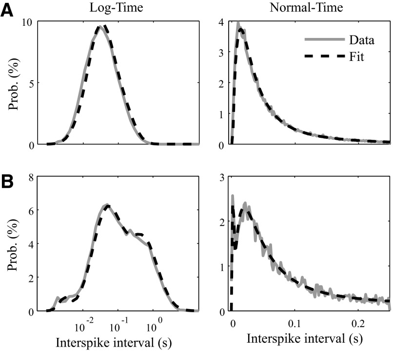
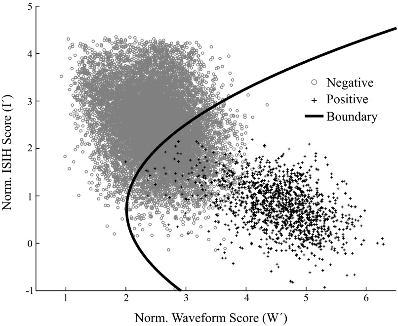
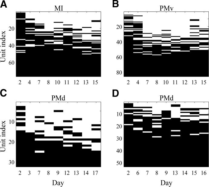
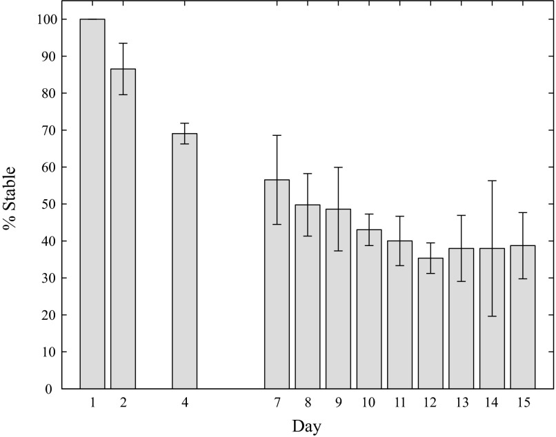
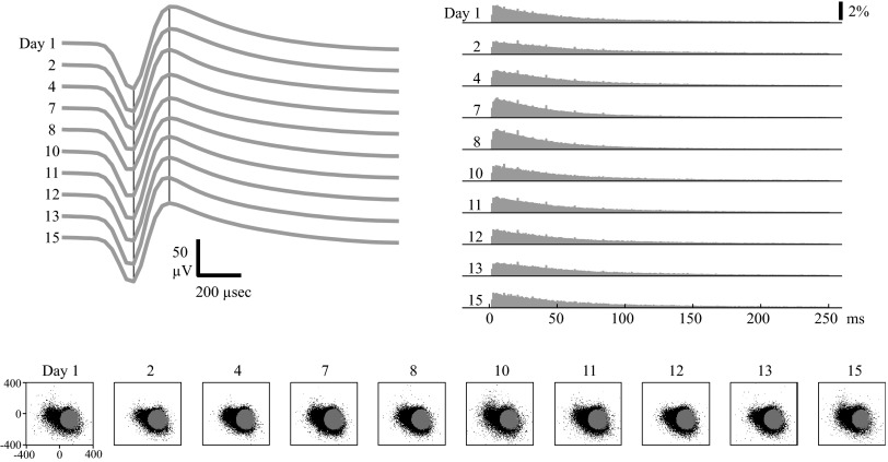
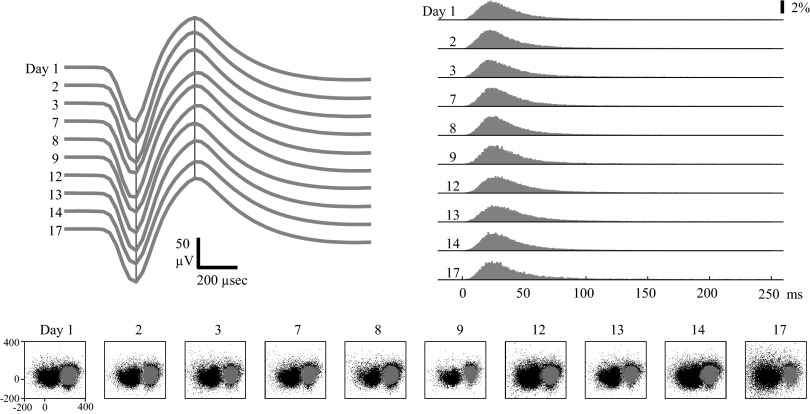
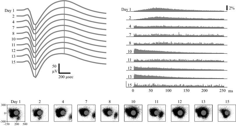
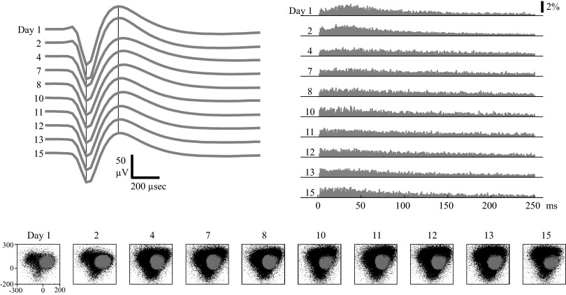
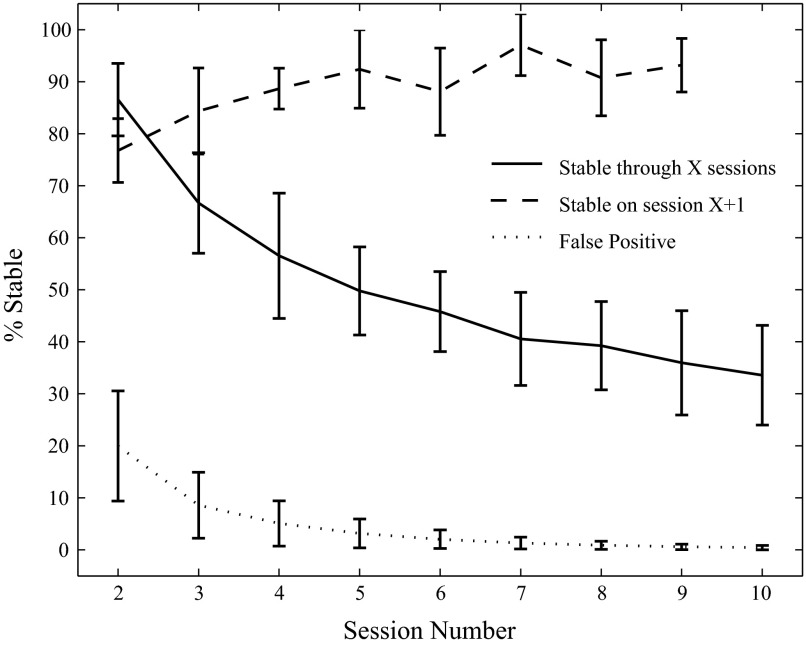
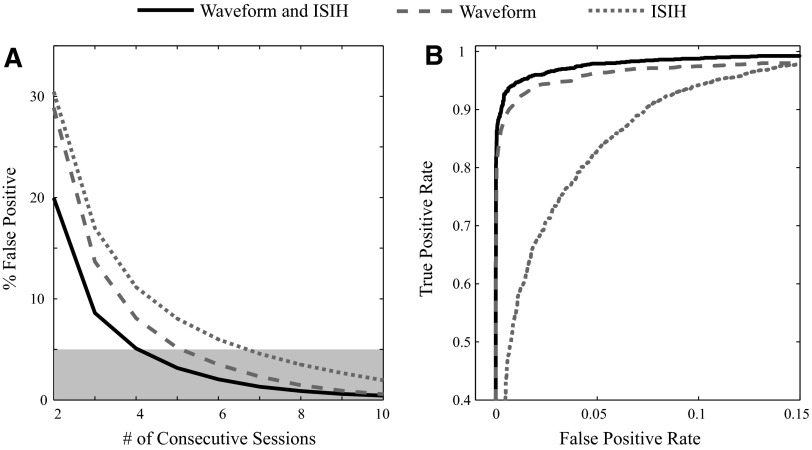
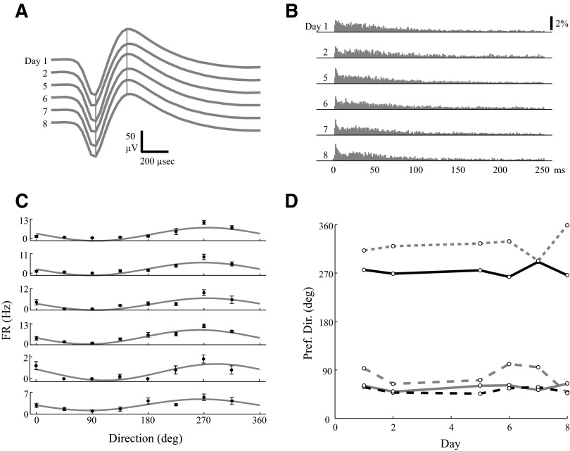
The use of chronic intracortical multielectrode arrays has become increasingly prevalent in neurophysiological experiments. However, it is not obvious whether neuronal signals obtained over multiple recording sessions come from the same or different neurons. Here, we develop a criterion to assess single-unit stability by measuring the similarity of 1) average spike waveforms and 2) interspike interval histograms (ISIHs). Neuronal activity was recorded from four Utah arrays implanted in primary motor and premotor cortices in three rhesus macaque monkeys during 10 recording sessions over a 15- to 17-day period. A unit was defined as stable through a given day if the stability criterion was satisfied on all recordings leading up to that day. We found that 57% of the original units were stable through 7 days, 43% were stable through 10 days, and 39% were stable through 15 days. Moreover, stable units were more likely to remain stable in subsequent recording sessions (i.e., 89% of the neurons that were stable through four sessions remained stable on the fifth). Using both waveform and ISIH data instead of just waveforms improved performance by reducing the number of false positives. We also demonstrate that this method can be used to track neurons across days, even during adaptation to a visuomotor rotation. Identifying a stable subset of neurons should allow the study of long-term learning effects across days and has practical implications for pooling of behavioral data across days and for increasing the effectiveness of brain-machine interfaces.

FIG. 1.

A mixture of 3 log-normals fits the interspike interval histograms (ISIHs) of 2 example neurons (A, top; B, bottom). Raw ISIHs are displayed in gray, whereas the fit traces are displayed in black, dashed lines. ISIHs are displayed both in normal time (right) and log-time (left). Note that the ISIH in B requires a mixture of 3 log-normals for a good fit, whereas the ISIH in A seems to be well fit with a single log-normal distribution (the expectation–maximization algorithm set the mixing probabilities of the other 2 log-normals close to zero).

FIG. 2.

Truly stable and truly unstable units are classified using a quadratic decision boundary. The normalized waveform scores (W′) and normalized ISIH scores (I′) are plotted for the true positive (i.e., truly stable; black crosses) and true negative (i.e., truly unstable; gray circles) data points. These scores were combined to create a quadratic decision boundary (black solid line), so that all data points falling to the right of the boundary were classified as stable.

FIG. 3.

Application of the stability criterion to 4 data sets. A black line segment indicates that the unit was stable on a given day relative to the first, reference day, whereas a blank, white line segment denotes that the unit was unstable. Note the x-axis shows the days of the recording sessions of each data set. A and B correspond to data sets from MI (A) and PMv (B) in monkey VL. C and D correspond to data sets from PMd in monkey BO (C) and monkey RJ (D). The unit indices are ordered from least stable (over all days) to most stable. MI, primary motor cortex; PMd, dorsal premotor cortex; PMv, ventral premotor cortex.

FIG. 4.

Percentage of stable units through a given day. The bar and error bar heights represent the mean and SD of the percentage of stable units over all data sets. Days that had one or no data points were left blank. All units were assumed to be stable on the first day.

FIG. 5.

Example of a stable MI unit. Top left: average waveforms from each session. The black vertical lines mark the peak and valley times of the first day's average spike waveform. Top right: ISIHs from each session. Bottom: unsorted (black) and sorted (gray) waveforms from each session projected onto the first (x-axis) and second (y-axis) principal components (PCs), as determined from the first session's data. The numbers ranging from 1 to 15 label the day each session was recorded on, relative to the first day. The ranges of axes (1st and 2nd PC coefficients) are labeled for the first day; subsequent days use the same axes.

FIG. 6.

Example of a stable PMd unit. Format is identical to that in Fig. 5. Note that there is a second waveform cluster (black dots) in PC space to the left of the sorted unit.

FIG. 7.

Example of a PMv unit with stable spike waveforms but unstable ISIHs. Format is identical to that in Fig. 5. The waveform criteria classified the unit as stable through day 13. However, the stability criteria (using both waveform and ISIH data) classified the unit as stable through day 2 but as unstable thereafter. Note the change in the ISIH between day 2 and day 4.

FIG. 8.

Example of an MI unit with unstable waveforms but stable ISIHs. Format is identical to that in Fig. 5. The ISIH criteria classified the unit as stable through day 15. However, the stability criterion classified the unit as stable through day 2 but as unstable thereafter. Note the change in waveform shape between day 2 and day 4.

FIG. 9.

Stable units are more likely to remain stable. The solid trace plots the percentage of the original units stable through a given number of consecutive sessions. With respect to the neurons that were stable through a given session, the dashed trace plots the percentage that were also stable on the next recording session. The dotted trace shows the estimated false-positive rate of classifying a unit as stable through a given number of sessions. The false-positive rate is derived by comparing units across different electrodes and seeing what percentage was classified as stable (see methods for details).

FIG. 10.

Using both waveform and ISIH data reduces false positives. A: the estimated false-positive rate, which is the percentage of units of the “true negatives” deemed to be stable through a given number of sessions, is less when using both waveform and ISIH data (solid black trace) than when using just waveform data (dashed gray trace) or just ISIH data (dotted gray trace) alone. The 5% significant level is also indicated (light gray box). The number of consecutive electrodes is used as a proxy for the number of sessions. B: the area under the receiver operating characteristic curve (a measure of classification performance) is higher when using both waveform and ISIH data then when using just waveform or just ISIH data alone. The differences in the area under the curves were found to be statistically significant (see text for details).

FIG. 11.

Stable units can be identified using only the prelearning epoch during an adaptation experiment. A: average waveforms of a stable MI unit across 6 sessions recorded over an 8-day period. B: ISIHs for the same unit. Formats for A and B are identical to the top of Fig. 5. C: this same unit shows a consistent directional tuning of the average (black dot, ±SE) firing rates in each direction and a consistent preferred direction of the fit (gray trace) cosine tuning curve. D: the preferred directions vs. the day of each recording session is plotted for 5 (of 25 total) units that displayed significant (P < 0.01) directional tuning on 6/6 sessions, including the unit from A–C (solid black trace).

References

1. Chen D, Fetz EE. Characteristic membrane potential trajectories in primate sensorimotor cortex neurons recorded in vivo. J Neurophysiol 94: 2713–2725, 2005. - PubMed
1. Georgopoulos AP, Schwartz AB, Kettner RE. Neuronal population coding of movement direction. Science 233: 1416–1419, 1986. - PubMed
1. Hastie T, Tibshirani R, Friedman J. The Elements of Statistical Learning: Data Mining, Inference, and Prediction. New York: Springer, 2001.
1. Hatsopoulos NG, Ojakangas CL, Paninski L, Donoghue JP. Information about movement direction obtained from synchronous activity of motor cortical neurons. Proc Natl Acad Sci US A 95: 15706–15711, 1998. - PMC - PubMed
1. Hatsopoulos NG, Xu Q, Amit Y. Encoding of movement fragments in the motor cortex. J Neurosci 27: 5105–5114, 2007. - PMC - PubMed
Publication types
LinkOut - more resources