Accuracy and precision in quantitative fluorescence microscopy

Abstract

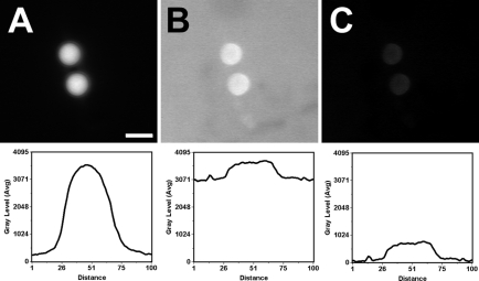
The light microscope has long been used to document the localization of fluorescent molecules in cell biology research. With advances in digital cameras and the discovery and development of genetically encoded fluorophores, there has been a huge increase in the use of fluorescence microscopy to quantify spatial and temporal measurements of fluorescent molecules in biological specimens. Whether simply comparing the relative intensities of two fluorescent specimens, or using advanced techniques like Förster resonance energy transfer (FRET) or fluorescence recovery after photobleaching (FRAP), quantitation of fluorescence requires a thorough understanding of the limitations of and proper use of the different components of the imaging system. Here, I focus on the parameters of digital image acquisition that affect the accuracy and precision of quantitative fluorescence microscopy measurements.

Figure 1.

Background fluorescence decreases precision of fluorescence intensity measurements. (A–C) Wide-field images of 6-µm fluorescent beads, all displayed with the same scaling so relative intensity is evident. All images were collected with the same microscope (model TE2000U; Nikon) and the same camera (ORCA-AG; Hamamatsu Photonics) using a Plan-Apochromat 60x 1.4 NA oil objective lens (Nikon) and MetaMorph software. (A) Fluorescent beads (mounted in PBS) with minimal background fluorescence. A 400-ms exposure time was used, and the maximum intensity value of the beads is ∼3,800. Bar = 5 µm. (B) A solution of fluorophore (with the same spectral characteristics as the fluorophore in the bead, diluted in PBS) was added to the specimen to increase the background fluorescence. The exposure time had to be decreased to 100 ms to get the same maximum intensity value of the beads, ∼3,800. (C) Image B, after background subtraction. Because a shorter exposure time was used in B, fewer photons from the beads were collected than in A. Collecting fewer photons from the object of interest means a higher contribution of Poisson noise, and less precise quantitation of fluorescence intensity values. Therefore, one should work to remove background fluorescence from the image (see Table I) before background subtraction.

Figure 2.

The importance of SNR in intensity and spatial measurements. (A) A digital image taken with a cooled CCD camera (ORCA-AG; Hamamatsu Photonics), with no light sent to the camera. Using MetaMorph software, a line (shown in red) was drawn across the bead and a line-scan graph was generated to show the intensity value of the pixels along the line. The graph shows line-scans of two similar images, taken in quick succession. The intensity values in the images fluctuate (range, 195–205) around the camera digital offset value of 200. Notice that the fluctuation in intensity values changes at each pixel from one image to the next. This variance is due primarily to thermal and readout noise from the CCD camera, and the extent of the variance will differ depending on the camera. This type of noise is superimposed on every fluorescence microscopy image. (B–E) Images of 6-µm beads that are fluorescently stained along their perimeter were collected with a wide-field microscope (model TE2000U; Nikon) using a Plan-Apochromat 60x 1.4 NA oil objective lens, the same camera as in A (ORCA-AG; Hamamatsu Photonics), and MetaMorph software. Line-scans generated as described for A. (B) An image of the bead taken with a 100-ms exposure time. The SNR is very low, making the bead indistinguishable from the noise in the line scan. (C) An image of the same bead as in B, taken with a longer (3 s) exposure time. The high SNR of this image would make quantitation of the intensity of the bead, or localization of the edge of the bead, highly precise. (D and E) The same bead images in B and C. Two images of the bead were taken, and one copy pseudo-colored red and one copy pseudo-colored green. The pseudo-colored images were shifted relative to one another by a few pixels and merged. (D) With low SNR images, it is nearly impossible to precisely locate the edges of the beads. (E) With high SNR images, the intensity line scan can be fit to Gaussian curves and the center located with nanometer precision. This allows the distance between objects of two wavelengths to be precisely determined, even if it is well below the resolution limit of the microscope (Churchman et al., 2005; Yildiz and Selvin, 2005; Huang et al., 2008; Manley et al., 2008). Bar = 5 µm.

Figure 3.

Resolution and sampling. (A–C) Images of the same pair of 150-nm green fluorescent beads collected with a microscope (model TE2000U; Nikon), a Plan-Apochromat 100x 1.4 NA oil objective lens, and MetaMorph software. A camera with 6.45-µm photodiodes (ORCA-AG; Hamamatsu Photonics) was used, and different camera binning settings were used to vary the area of the specimen covered by one pixel. Exposure times were adjusted to reach a maximum intensity value of ∼3,600 for each image. Using the equation for lateral resolution, we can calculate that the diameter of the first minimum of the airy disk, and therefore the diameter of the bead in the optical image, should be equal to ∼465 nm. Bar = 0.5 µm. (A) An image collected with no camera binning, and an exposure time of 200 ms. Each pixel corresponds to ∼65 nm of the specimen, and each bead is sampled with ∼7 pixels. (B) An image collected using 2 × 2 camera binning, and an exposure time of 50 ms. Each pixel corresponds to ∼129 nm of the specimen, and each bead is sampled with about 3.5 pixels. (C) An image collected using 4 × 4 camera binning, and an exposure time of 25 ms. Each pixel corresponds to ∼258 nm of the specimen, and each bead is sampled with less than 2 pixels. The optical image is under-sampled, and the two beads can no longer be distinguished as separate from one another.

Figure 4.

Non-uniform illumination results in nonuniform fluorescence. All images were collected using a microscope (model TE2000E; Nikon), a Plan-Apochromat 20x 0.75 NA objective lens, a camera (ORCA-AG; Hamamatsu Photonics), and MetaMorph software. (A) An image of a field of fluorescent beads, using wide-field illumination. Individual beads contain a similar concentration of fluorophore (clumps of beads appear brighter, as is seen near the center of the image). A pseudo-color displaying the range of intensity values (see inset) was applied. Note that beads in the top left have different intensity values than the beads in the bottom right. (B) An image of a uniform field of fluorophore taken with the same microscope optics and conditions as A, showing uneven illumination across the field of view. This nonuniform illumination explains the nonuniform fluorescence from the beads of similar fluorophore concentration shown in A. (C) After flat-field correction (Zwier et al., 2004; Wolf et al., 2007), the image intensity values more accurately reflect the real fluorescence in the specimen. This image was obtained using the image arithmetic function in image processing software (in this case, MetaMorph) to divide the image in A by the image in B. Bar = 50 µm.

Figure 5.

Bleed-through can cause inaccuracy in intensity measurements. (A and B) Images of a cell (outlined in white) labeled with DAPI (nuclei) and Bodipy-FL phalloidin (actin). Both images were collected using the same microscope (model 80i; Nikon), a Plan-Apochromat 100x NA 1.4 oil objective lens, the same camera (ORCA R2; Hamamatsu Photonics), and MetaMorph software. The same camera acquisition settings were used for both images, but they were collected using two different filters designed for imaging DAPI. (A) An image collected with a DAPI filter set containing a long-pass emission filter, which allows bleed-through of the Bodipy-FL signal in the cytoplasm. The bleed-through of the actin in the cytoplasm is just barely visible by eye in the image. The average intensity value of the cytoplasm in this image is 205. (B) An image of the same cell as in A, collected with a DAPI filter set containing a band-pass emission filter, which blocks bleed-through of the Bodipy-FL signal in the cytoplasm. The average intensity value of the cytoplasm in this image is 91, over 50% less than the image in A. Bar = 10 µm.

Figure 6.

Shifts in image registration can affect colocalization results. (A and B) Images of 100-nm Tetra-Speck beads (Invitrogen; mounted in glycerol) that fluoresce multiple colors including red and green, collected with a microscope (model 80i; Nikon) and camera (ORCA R2; Hamamatsu Photonics) using a Plan-Apochromat 100x NA 1.4 oil objective lens and MetaMorph software. One image of the beads was collected using a filter set for green fluorescence (FITC) and a second image of the beads was collected using a filter set for red fluorescence (TRITC); all other microscope optics were the same between the two images. The two images were pseudo-colored and merged using MetaMorph software. The scatter plots (generated in MetaMorph) display the correlation between the intensity values of the red and green pixels in the images. (A) The merged image, showing a registration shift of several pixels between the red and green images. 10 sets of images were collected to determine that the shift is repeatable, and therefore most likely caused by the filter sets (not depicted). The correlation coefficient for these red and green images is only 0.72, even though the red and green images represent the exact same beads. Bar = 1 µm. (B) The same images as in A, after correction for the shift in registration using MetaMorph image processing software. The correlation coefficient increased to 0.97 after the correction.

References

1. Adams M.C., Salmon W.C., Gupton S.L., Cohan C.S., Wittmann T., Prigozhina N., Waterman-Storer C.M. 2003. A high-speed multispectral spinning-disk confocal microscope system for fluorescent speckle microscopy of living cells.Methods. 29:29–41 - PubMed
1. Allan V.J. 2000. Protein Localization by Fluorescence Microscopy: A Practical Approach. Oxford University, New York: 256 pp
1. Art J. 2006. Photon detectors for confocal microscopy. Handbook of Biological Confocal Microscopy. Pawley J.B., editor Springer-Verlag New York, Inc., New York: 251–262
1. Aubin J.E. 1979. Autofluorescence of viable cultured mammalian cells.J. Histochem. Cytochem. 27:36–43 - PubMed
1. Axelrod D., Thompson N.L., Burghardt T.P. 1983. Total internal inflection fluorescent microscopy.J. Microsc. 129:19–28 - PubMed