Optical imaging of contextual interactions in V1 of the behaving monkey

Abstract

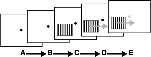
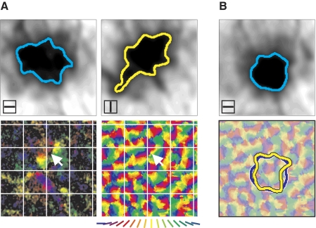
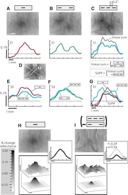
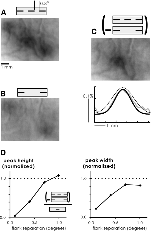
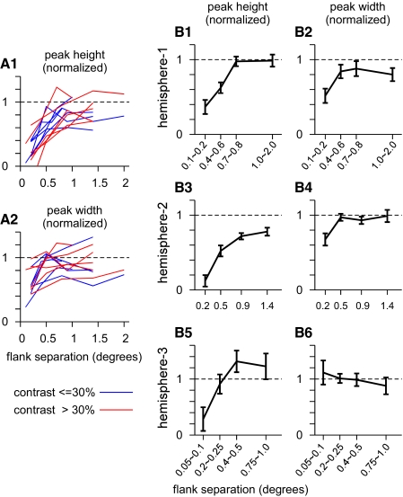
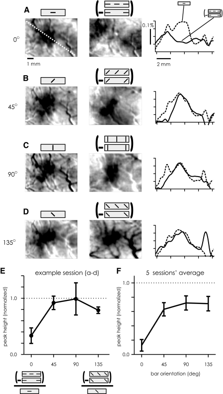
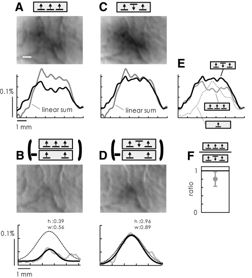
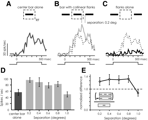
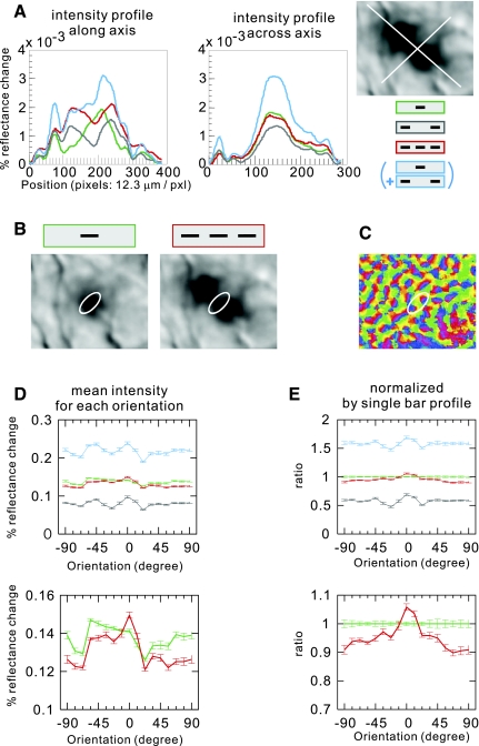
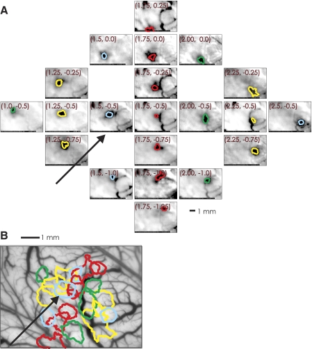
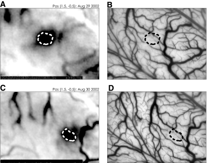
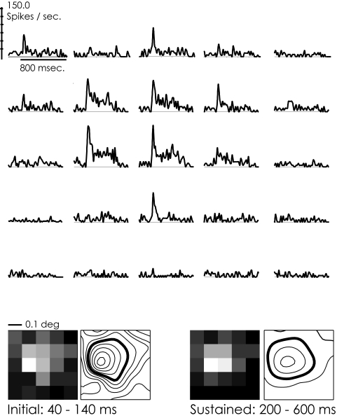
Interactions in primary visual cortex (V1) between simple visual elements such as short bar segments are believed to underlie our ability to easily integrate contours and segment surfaces. We used intrinsic signal optical imaging in alert fixating macaques to measure the strength and cortical distribution of V1 interactions among collinear bars. A single short bar stimulus produced a broad-peaked hill of activation (the optical point spread) covering multiple orientation hypercolumns in V1. Flanking the bar stimulus with a pair of identical collinear bars led to a strong nonlinear suppression in the optical signal. This nonlinearity was strongest over the center bar region, with a spatial distribution that cannot be explained by a simple gain control. It was a function of the relative orientation and separation of the bar stimuli in a manner tuned sharply for collinearity, being strongest for immediately adjacent bars lying on a smooth contour. These results suggest intracortical interactions playing a major role in determining V1 activation by smooth extended contours. Our finding that the interaction is primarily suppressive when imaged optically, which presumably reflects the combined inhibitory and excitatory inputs, suggests a complex interplay between these cortical inputs leading to the collinear facilitation seen in the spiking response of V1 neurons. This disjuncture between the facilitation seen in spiking and the suppression in imaging also suggests that cortical representations of complex stimuli involve interactions that need to be studied over extended networks and may be hard to deduce from the responses of individual neurons.

FIG. 1.

Sequence for one imaging cycle: the trial starts with the animal pulling a lever, displaying a fixation spot (A). Once the animal has achieved fixation (B), the initial “blank screen” baseline optical image is acquired for 2–4 image frames each 400 ms in duration. The visual stimulus (grating or bar) is then flashed on (C); it remains stationary for one to two 400-ms frames before starting to drift (D). The animal has to maintain fixation until the fixation spot dims (E) after four to eight 400-ms frames, 1.6–3.2 s.

FIG. 2.

Reducing vascular artifacts by aligning all image frames to first frame. A: single normalized image frame (image frame divided by “blank screen” base reference frame) without shifting individual frames into alignment. B: same normalized image after aligning each component frame to a common template. C: ocular dominance image obtained without aligning frames. Small relative movements between “right eye” and “left eye” frames acts as an “edge enhancer,” throwing vasculature into high relief. D: same ocular dominance image after aligning all frames with a common template.

FIG. 3.

Horizontal and vertical axes mapped on primary visual cortex (V1), 1° spacing. A: visuotopic V1 map of vertical axes, optically imaged with vertical “candy-stripe” stimulus consisting of 0.5°-wide vertical strips of drifting grating, alternating with strips of neutral gray. B: visuotopic V1 map of horizontal axes, obtained with a horizontal “candy stripe” stimulus. Note that the edge of the grating is visible (bottom right). C: mapping absolute visuotopic axes (vertical) on V1. Individual visuotopic images of vertical stripes on V1 were joined into a mosaic using vascular landmarks to blanket the central imageable area of the craniotomy. The absolute x-coordinates of individual lines (broken line) were obtained by comparing with the optical images of small single stimulus bars at positions defined with respect to the monkey's fixation point. The “candy-striped” grating pattern is schematically drawn as the inset. D: absolute visuotopic horizontal axes; same as C but horizontal stripes. The absolute y-coordinates are indicated by broken lines. Each image in this figure consisted of 58–190 recording trials.

FIG. 4.

Fitting tilted baseline to point spread images. A: schematic showing the effect of adding a tilted baseline to a model Gaussian point spread. B: raw point-spread image showing distinct gradient of darkening in the baseline toward the top left. C: regression plane is fitted to the part of the image lying outside the dashed circle. D: the fitted plane. E: image after subtracting the regression plane. (All images are on the same gray scale.)

FIG. 5.

Optical images, i.e., optical point spreads generated by 0.5 and 0.25° stimulus bars. A: point spreads generated by 0.5° bar. Top left: horizontal bar drifting vertically back and forth over a 0.5° region. Top right: vertical bar drifting horizontally. Contours mark 50% image density. Bottom left: local optical map obtained by combining optical point spreads from bars at 4 orientations—0, 45, 90, and 135°—into a “polar” map of orientation with hue encoding orientation preference (see key below) and brightness proportional to vector signal strength (Das and Gilbert 1995). Bottom right: orientation map obtained using full-field drifting gratings from the same region of V1. Note the match with the local orientation map around the arrowhead. Grid at 1-mm spacing is superimposed for ease of comparison. B: point spreads generated by 0.25° bar. Top: horizontal bar moved back and forth vertically over 0.25°. Bottom: the 50% contour (blue) is superimposed over the full orientation map, along with the 50% contour for the point spread from a 0.25° vertical bar drifted horizontally (yellow). The background orientation map is the same as that in A, bottom right map, but its color saturation is reduced for emphasizing the contour lines. Two contour lines were well overlapped in 0.25° bar-width condition.

FIG. 6.

Flanking collinear bars suppress the optical point spread from a single bar. A, top image: optical point spread from a single 0.25° bar (horizontal bar as indicated by key above, 20% contrast, drifting back and forth over 0.25°). Image density encodes optical signal strength (i.e., percentage change in cortical reflectance) as shown in gray scale key below. Bottom graph: cross-sectional profile at S1 (see inset D). (Scale bars: in image, bar: 1 mm; for profile, x-axis scale bar = 1 mm, y-axis scale bar = 0.1% cortical reflectance change.) B: optical image and signal strength profile from flanks alone. C: optical image and signal strength profile (blue line) from 3-bar array; bar separation = 0.2°. The gray line profile represents the “linear sum” of the response profiles of the single-bar (A) and the flanks-alone (B). D: the contours for cross-sectional profiles shown in A–C and G (S1), E (S2: cross section at center bar location), and F (S3: cross section at the flanks). On each profile, signal strength was averaged over about 0.4-mm width across the broken line. E: cross-sectional profiles at S2. Blue line: 3-bar array; red line: single bar. F: cross-sectional profiles at S3. Blue line: 3-bar array; green line: flanks alone. G: the profile of collinear suppression (black line: “SUPP” defined as “linear sum” minus “3-bar”). H, top: single-bar optical point spread, same as in A. The box below shows 3-dimensional (3D) perspectives of the same image and of the Gaussian fitted to the optical image by least squares. The inset shows the cross-sectional profile through the fitted Gaussian (black) superimposed on a cross section of the image (gray). I, top: difference image obtained by subtracting “flanks alone” (B) from “3-bar image” (C). Bottom: 3D perspectives of this difference image and the fitted Gaussian. Inset: profiles through image and fitted Gaussian. Gaussian height and width as fractions of the single-bar Gaussian fit (shown as thin dashed line). All scale bars as in A: i.e., horizontal: 1 mm, vertical: 0.1% cortical reflectance change. Each image in this figure is the average of 13–16 recording trials.

FIG. 7.

Flank suppression drops with increasing bar separation: A: optical signal from 3-bar array, with center bar of the same size and location as in Fig. 6, but with flank bar separation = 0.8°. B: flanks alone. C, top: difference image for 0.8° bar separation (A minus B). Bottom: Gaussian (black) fitted to difference image (gray) with height; width measured as fraction of single-bar Gaussian fit (shown as thin dashed line). D: an example response profile of one recording session. Left: suppression of peak height as a function of flank separation. Heights of Gaussians fitted to difference images, normalized by the height of single-bar Gaussian fit. Right: suppression of peak width as a function of flank separation. Widths of fitted Gaussians similarly normalized to single-bar Gaussian width. (Normalized value = 1 implies no nonlinear suppression; 0: full suppression. Error bar represents SE.) Each image in this figure is the average of 8–15 recording trials.

FIG. 8.

Population results of the signal suppression depending on the bar separation. Summarized results recorded from 3 hemispheres. A1: normalized peak heights are plotted against the bar separation. Each curve represents a result taken from one recording session. In each recording session, each stimulus condition was repeated ≥8 trials (in most case repeated >10 trials). The blue curve represents the result of a low-contrast (≤30%) stimulus condition. The red curve represents a high-contrast (>30%) condition. In any contrast condition, the response profiles were similar. The stronger suppression is observed at the closer bar separation. Eccentricities of the recording sites were between 3.6 and 4.6°. These data were recorded from hemisphere 1 (B1) and hemisphere 2 (B3). The error bar was omitted in this plot for visibility of the graph. A2: normalized peak width for each recording session. Other conditions are the same as in A1. B1, B3, B5: averaged normalized peak heights. B2, B4, B6: averaged normalized peak width. B1, B2: averaged data recorded from hemisphere 1 (monkey 1). Five recording sessions (recorded in 3 days) were averaged. Eccentricities of the recording sites were between 3.6 and 4.6°. Stimulus bar length was 0.25°. Stimulus contrasts were between 20 and 80%. B3, B4: data from hemisphere 2 (monkey 2) averaged from 7 recording sessions (recorded in 3 days). Eccentricity was 4.3°. Bar length was 0.25°. Contrasts were between 20 and 60%. B5, B6: data from hemisphere 3 (monkey 2) averaged from 9 recording sessions (recorded in 3 days). Eccentricities were between 1.6 and 1.9°. Bar length was 0.2°. Contrasts were between 65 and 85%. The abscissa of each graph represents the bar separation in degrees. Each error bar in B1–B6 represents SE across the sessions.

FIG. 9.

Flank suppression is orientation specific. A (“0°”), left: optical point spread from a single 0.5° horizontal bar. Center: difference image, obtained by subtracting optical image due to collinear flanks alone from image due to a horizontal array of 3 collinear horizontal bars moving in synchrony (stim contrast: 90%; flanks at separation: 0.1°). Right: signal strength profiles along the diagonal line (white broken line on the left image). Broken line curve: profile for single bar; solid line curve: difference image. [Scales: image: 1 mm. Graph: abscissa: 2 mm; ordinate: 0.1% cortical reflectance change. Image is shown at saturated contrast.] B (“45°”): same as top row, but for stimulus bars oriented at 45°. The center bar and flank bars had the same center positions as those in the horizontal bar stimuli in the top row. The signal profiles (right) were also taken at the same diagonal line shown in A. C (“90°”) and D (“135°”): same as 2nd row, but with 90 and 135° bars, respectively. E: one recording session example of heights of Gaussians fitted to difference images (A–D, center), normalized in each case to the corresponding single-bar Gaussian fitted to a single-bar image (A–D, left), as a function of stimulus bar orientation. (Fitted Gaussians are not shown, but it was calculated as indicated in Fig. 6, H and I.) The error bar represents SE. Number of trials were 11–13 for each orientation condition. F: the averaged Gaussian heights over multiple recording sessions, as a function of bar orientation. The error bar represents SE. Five recording sessions (in 4 days) were performed on 2 monkeys. Stimulus contrasts ranged from 80 to 90%. The eccentricities ranged from 1.7 to 4.2°. The bar lengths ranged from 0.2 to 0.5°.

FIG. 10.

Suppression by flanks moving in phase and in counterphase with central bar. A: 3-bar optical image and its cross-sectional profile (black line). Same experiment as in Fig. 6. The gray line profile represents the “linear sum” of the response profiles of the single-bar and the flanks-alone (same as Fig. 6C, shown again for ease of comparison). B: corresponding difference image, signal profile, and fitted Gaussian (same as Fig. 6I). C: 3-bar image but with flanks moving in counterphase to the center bar and its cross-sectional profile. Black line: counterphase profile. Gray line: “linear sum.” D: difference image for 3-bar counterphase array, signal profile, and fitted Gaussians; heights and widths normalized to those for single-bar image (thin dashed line). Scale bars as in Figs. 6 and 7: horizontal bar = 1 mm; vertical = 0.1% change in cortical reflectance. E: comparison of the cross-sectional profiles. Black line: counterphase 3-bar (C). Solid gray line: in-phase 3-bar (A). Broken gray line: single-bar (Fig. 6A). The strongest signal was seen in the counterphase stimulus. This means that both in-phase 3-bar and single-bar optical signal were not saturated. All cross-sectional profiles in this figure were measured at S1 location indicated in Fig. 6D. F: population data for the relationship between in-phase signal strength and counterphase strength. The signal strength was measured in the region around the peak position of the single-bar image (width 0.5–1.0 mm) and averaged for each stimulus condition (each condition was repeated for 11–20 trials). The in-phase signal strength was normalized by the maximum counterphase signal in the same recording session. The average of 44 in-phase condition data are plotted. The error bar represents SD. Each image in this figure is the average of 11–14 recording trials.

FIG. 11.

In electrode recordings, collinear flanks facilitate suprathreshold spiking responses of V1 neurons. An example of single-neuron response. A, dark gray: peristimulus time histogram (PSTH) of spiking response to single bar at the preferred orientation of the recorded neuron. B, light gray: the response to the single bar is facilitated by collinear flanks that do not, by themselves, stimulate the neuron (C). Dashed line shows the response to the single bar, for comparison; bar below PSTH indicates stimulus duration. D: neuron response to single bar (dark gray) and to 3-bar (light gray) as a function of the separation between flanks and center (PSTH averaged over the time interval 100–400 ms after stimulus onset). The facilitation by the collinear flanks is strongest at the closest approach between flanks and center. The t-test was significant (P < 0.01) for comparison between “center bar alone” and each of 0.2, 0.4, 0.6, and 0.8° separation and not significant between “center bar alone” and 1.0° separation. The error bar represents SE. Number of trials was 11–12 for each condition. E: normalized differential response, which was calculated as in Fig. 7D. Flanks-alone response was subtracted from 3-bar response and this difference was divided by the single-bar response.

FIG. 12.

Suppression of three-bar optical imaging signal relative to the linear sum is not explained by selective orientation-tuned suppression induced by the flanks. A: profile of signal intensity along test lines lying along (left) or across (middle) the axis of the 3-bar image. Color coded as shown (green: single-bar; gray: flanks alone; red: 3-bar; blue: linear sum). Test lines shown on inset image (of 3-bar response). B: ROIs for calculating orientation tuning, shown on a single-bar and 3-bar image. C: ROI aligned over underlying orientation map. D: orientation tuning calculated within ROI for the different bar combinations (color code as in panel A). Top: shown with image scale starting from zero; bottom, scaled to magnify single-bar and 3-bar results. E: same, normalized to single-bar signal.

FIG. A1.

Precision of the fine-grained optical map of retinotopy. A: individual point spreads from 0.25° bars located on a grid with 0.25° spacing. We optically imaged V1 responses to single 0.25° stimulus bars (each drifting within a 0.25° region in visual space), centered at specified locations with respect to the fixation point. Here we show a (single day's) set of 21 individual optical images, each corresponding to a different bar center location (average ∼10 trials per location, interleaved). The images are arranged by stimulus position: neighboring positions represent a horizontal or vertical shift of 0.25° in visual space. [Images labeled by the bar location; gaps in the image: where the bar was shifted by 0.5°. Colored contours mark the 66% peak height. Arrow marks the point spread due to a stimulus bar centered at (1.5°, −0.5°); the same stimulus location is used again in Fig. A2.] B: neighboring stimuli 0.25° apart form distinct point spreads on cortex. All the 66% contours of individual point spreads shown in A are combined and superimposed on the vascular map of cortex. Note, for example, the well-separated set of contours (red) marking point spreads lying along the vertical axis at x = 1.75. The few irregular contours with large areas of overlap with their neighbors come from point-spread images distorted by large underlying blood vessels. Note: in this set of images we show the 66% contours rather than the 50% contours as in the main text, to get a sharp estimate of point-spread peaks. This also minimized the distortion of the outline by big blood vessel artifacts for the few images in which such artifacts were prominent (see position 2.25, −0.5).

FIG. A2.

Point spreads from a given spatial location superimpose closely on each other from day to day. A: point spread for stimulus at location (1.5, −0.5) with respect to the animal's fixation point (see arrow, Fig A1A). B: the contour from A, superimposed on the vascular map of cortex taken during the same imaging session. C: point spread for a stimulus bar at the same location (1.5, −0.5) with respect to the animal's fixation, imaged on a different day. The point spread appears shifted because of a slight shift in the camera position. D: the 66% contour from C, superimposed on the vascular map of cortex taken during the same recording session. The contour falls on the same location with respect to the underlying vascular map as the contour in B.

FIG. A3.

Two-dimensional (2D) receptive field (RF) histogram of extracellular spiking response, recorded with metal electrode through artificial dura. Top: individual PSTHs arranged by stimulus position (stimulus: 0.1° × 0.1° square flashed over a 5 × 5 grid with 0.1° spacing; 9 trials each position, randomly interleaved). Bottom: 2D RF profile, mapped as average spike rate for initial (40–140 ms) or sustained (200–600 ms) phase of neuron response. Contour maps were drawn using a smoothed surface spline-fit to 2D RF profile, with contours at 10 spikes/s steps. Contour at 50% peak (thick line) gives an RF dimension = 0.28° (full width at half-maximum).

References

1. Angelucci A, Levitt JB, Walton EJS, Hupe J-M, Bullier J, Lund J. Circuits for local and global signal integration in primary visual cortex. J Neurosci 22: 8633–8646, 2002. - PMC - PubMed
1. Bishop PO, Coombs JS, Henry GH. Receptive fields of simple cells in the cat striate cortex. J Physiol 231: 31–60, 1973. - PMC - PubMed
1. Blakemore C, Tobin EA. Lateral inhibition between orientation detectors in the cat's visual cortex. Exp Brain Res 15: 439–440, 1972. - PubMed
1. Blasdel G, Campbell D. Functional retinotopy of monkey visual cortex. J Neurosci 21: 8286–8301, 2001. - PMC - PubMed
1. Bonhoeffer T, Grinvald A. Optical imaging based on intrinsic signals: the methodology. In: Brain Mapping: The Methods (2nd ed.), edited by Toga AW, Mazziotta JC. San Diego, CA: Academic Press, 1996, p. 97–140.
Publication types
LinkOut - more resources