

doi: 10.1126/science.1174294.
Cell growth and size homeostasis in proliferating animal cells
Affiliations
- PMID: 19589995
- PMCID: PMC2905160
- DOI: 10.1126/science.1174294
Item in Clipboard
Cell growth and size homeostasis in proliferating animal cells
Science.
.
Abstract
A long-standing question in biology is whether there is an intrinsic mechanism for coordinating growth and the cell cycle in metazoan cells. We examined cell size distributions in populations of lymphoblasts and applied a mathematical analysis to calculate how growth rates vary with both cell size and the cell cycle. Our results show that growth rate is size-dependent throughout the cell cycle. After initial growth suppression, there is a rapid increase in growth rate during the G1 phase, followed by a period of constant exponential growth. The probability of cell division varies independently with cell size and cell age. We conclude that proliferating mammalian cells have an intrinsic mechanism that maintains cell size.
Figures
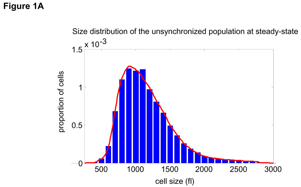
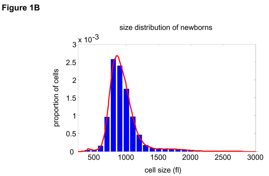
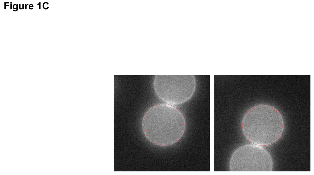
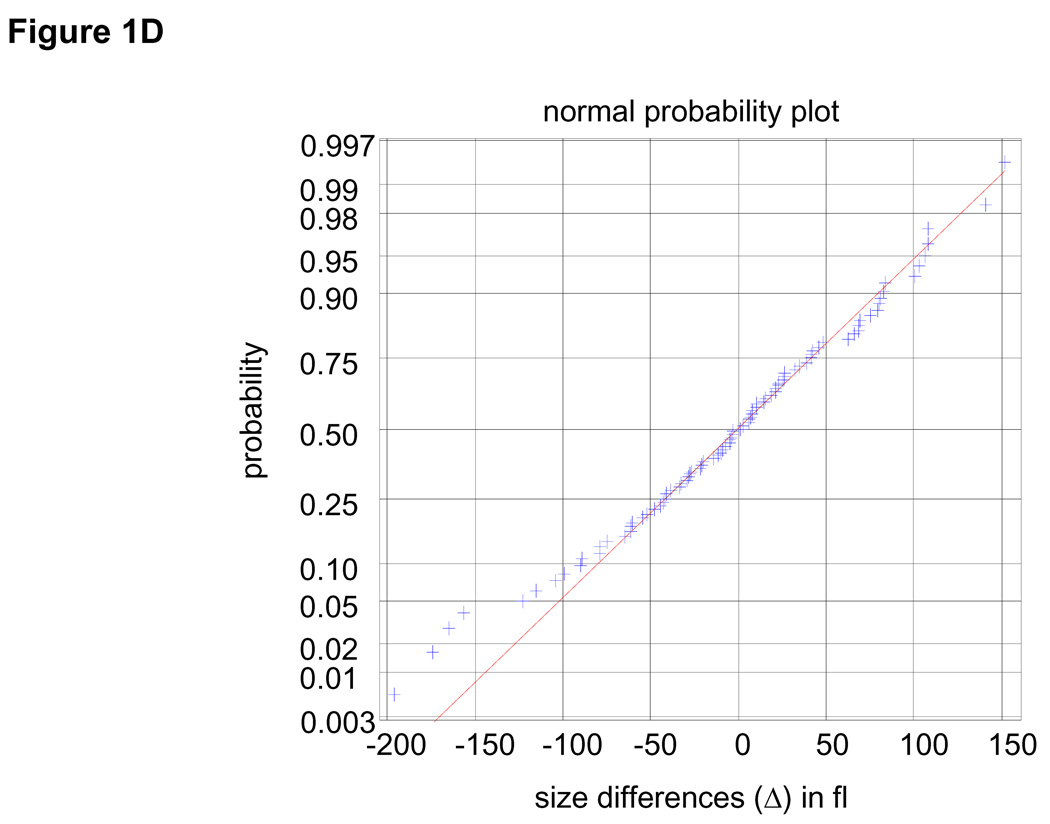
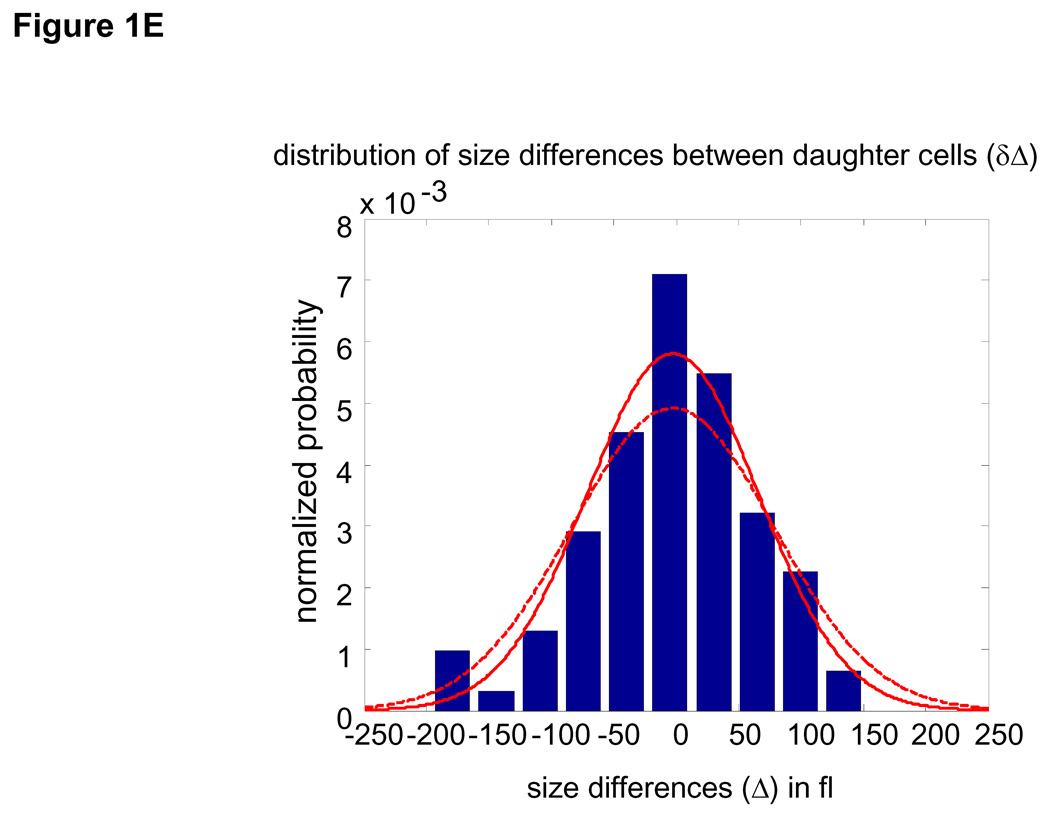
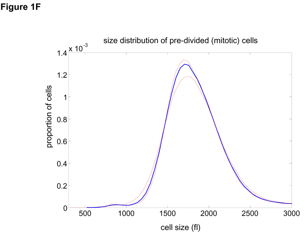
Size distribution of (A) asynchronous steady-state and (B) newborns populations are shown by histograms (blue) and kernel density estimates (red). (C) L1210 cells, membrane labeled with GFP were imaged while exiting mitosis. Each cell was fitted a circle at maximum diameter. See SOM for details and error (D) A quantile normal plot showing the normality of the daughter cell volume differences, Δ. (E) A single parameter for the variance, σ2, of the Gaussian estimate (red) for the distribution, δ(Δ). Also shown is the distribution corresponding to the upper confidence interval of the Gaussian estimate (dashed red). (F) Mitotic size distribution calculated by convolving newborn size distribution with δ(Δ). Confidence intervals of δ(Δ) distribution were utilized to generate the confidence of the mitotic size distribution (shown in red). See SOM for details.
Size distribution of (A) asynchronous steady-state and (B) newborns populations are shown by histograms (blue) and kernel density estimates (red). (C) L1210 cells, membrane labeled with GFP were imaged while exiting mitosis. Each cell was fitted a circle at maximum diameter. See SOM for details and error (D) A quantile normal plot showing the normality of the daughter cell volume differences, Δ. (E) A single parameter for the variance, σ2, of the Gaussian estimate (red) for the distribution, δ(Δ). Also shown is the distribution corresponding to the upper confidence interval of the Gaussian estimate (dashed red). (F) Mitotic size distribution calculated by convolving newborn size distribution with δ(Δ). Confidence intervals of δ(Δ) distribution were utilized to generate the confidence of the mitotic size distribution (shown in red). See SOM for details.
Size distribution of (A) asynchronous steady-state and (B) newborns populations are shown by histograms (blue) and kernel density estimates (red). (C) L1210 cells, membrane labeled with GFP were imaged while exiting mitosis. Each cell was fitted a circle at maximum diameter. See SOM for details and error (D) A quantile normal plot showing the normality of the daughter cell volume differences, Δ. (E) A single parameter for the variance, σ2, of the Gaussian estimate (red) for the distribution, δ(Δ). Also shown is the distribution corresponding to the upper confidence interval of the Gaussian estimate (dashed red). (F) Mitotic size distribution calculated by convolving newborn size distribution with δ(Δ). Confidence intervals of δ(Δ) distribution were utilized to generate the confidence of the mitotic size distribution (shown in red). See SOM for details.
Size distribution of (A) asynchronous steady-state and (B) newborns populations are shown by histograms (blue) and kernel density estimates (red). (C) L1210 cells, membrane labeled with GFP were imaged while exiting mitosis. Each cell was fitted a circle at maximum diameter. See SOM for details and error (D) A quantile normal plot showing the normality of the daughter cell volume differences, Δ. (E) A single parameter for the variance, σ2, of the Gaussian estimate (red) for the distribution, δ(Δ). Also shown is the distribution corresponding to the upper confidence interval of the Gaussian estimate (dashed red). (F) Mitotic size distribution calculated by convolving newborn size distribution with δ(Δ). Confidence intervals of δ(Δ) distribution were utilized to generate the confidence of the mitotic size distribution (shown in red). See SOM for details.
Size distribution of (A) asynchronous steady-state and (B) newborns populations are shown by histograms (blue) and kernel density estimates (red). (C) L1210 cells, membrane labeled with GFP were imaged while exiting mitosis. Each cell was fitted a circle at maximum diameter. See SOM for details and error (D) A quantile normal plot showing the normality of the daughter cell volume differences, Δ. (E) A single parameter for the variance, σ2, of the Gaussian estimate (red) for the distribution, δ(Δ). Also shown is the distribution corresponding to the upper confidence interval of the Gaussian estimate (dashed red). (F) Mitotic size distribution calculated by convolving newborn size distribution with δ(Δ). Confidence intervals of δ(Δ) distribution were utilized to generate the confidence of the mitotic size distribution (shown in red). See SOM for details.
Size distribution of (A) asynchronous steady-state and (B) newborns populations are shown by histograms (blue) and kernel density estimates (red). (C) L1210 cells, membrane labeled with GFP were imaged while exiting mitosis. Each cell was fitted a circle at maximum diameter. See SOM for details and error (D) A quantile normal plot showing the normality of the daughter cell volume differences, Δ. (E) A single parameter for the variance, σ2, of the Gaussian estimate (red) for the distribution, δ(Δ). Also shown is the distribution corresponding to the upper confidence interval of the Gaussian estimate (dashed red). (F) Mitotic size distribution calculated by convolving newborn size distribution with δ(Δ). Confidence intervals of δ(Δ) distribution were utilized to generate the confidence of the mitotic size distribution (shown in red). See SOM for details.
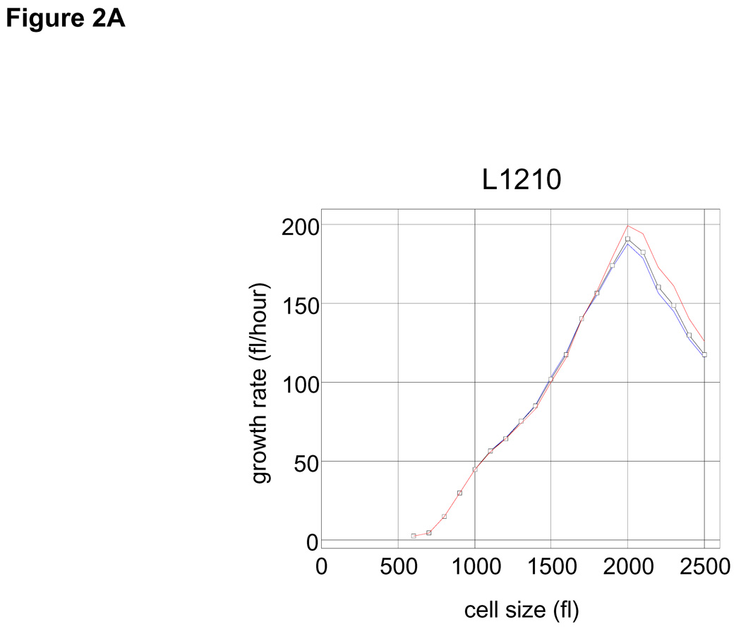
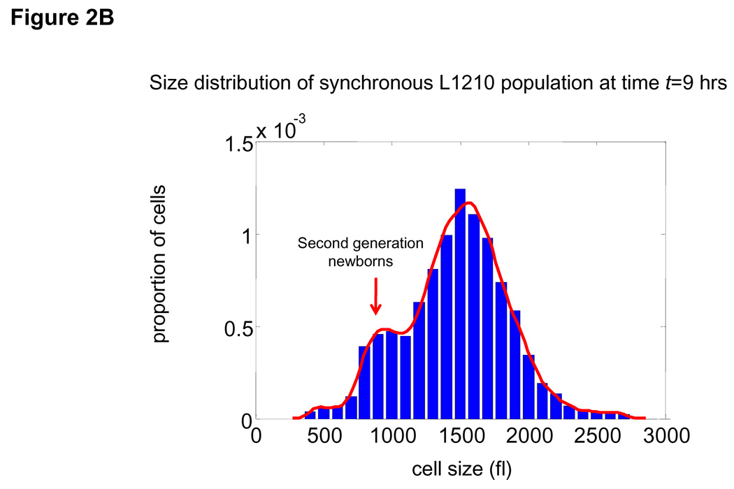
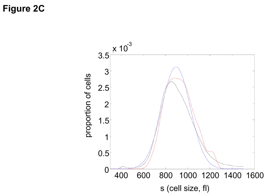
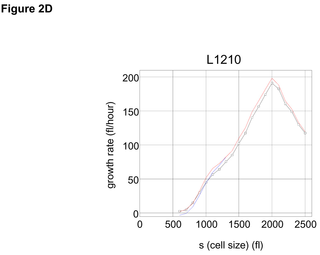
(A) Mean growth rate (fl/hour) is shown as a function of cell size (fl) for L1210 cells. Curve (black) was calculated from the Coulter Counter® measurements of asynchronous size distribution (106 cells), and the size distribution of newborns (105 cells) together with the daughter cell correlation (see Fig. 1) using the Collins-Richmond method. Also shown are the curves based on the assumption of symmetric division (blue) and on a variance for daughter cell differences that is 2 times higher than the measured value (red). Due to the large numbers of cells in the datasets, errors in growth rate obtained from this calculation are less than 1 fl/hour (see SOM). (B) Bimodal size distribution of synchronous L1210 population at time t = 9 hrs. The left mode represents second generation newborns generated completely in suspension. (C) The similarity in the size distribution of the newborns freshly eluted from membrane compared to the size distribution of newborns generated in suspension. The black line corresponds to the size distribution of eluted newborns. We calculate the size distribution of the second generation newborns (blue). The two size modes at t=9 hrs were separated using a Gaussian extrapolation. In red is an alternative extrapolation of the same distribution obtained by a method used later in the study to calculate the probabilities of cell division (see text). (D) Collins-Richmond growth plot (black) was recalculated using second generation newborns. Red and blue curves represent the different methods of extrapolating newborns.
(A) Mean growth rate (fl/hour) is shown as a function of cell size (fl) for L1210 cells. Curve (black) was calculated from the Coulter Counter® measurements of asynchronous size distribution (106 cells), and the size distribution of newborns (105 cells) together with the daughter cell correlation (see Fig. 1) using the Collins-Richmond method. Also shown are the curves based on the assumption of symmetric division (blue) and on a variance for daughter cell differences that is 2 times higher than the measured value (red). Due to the large numbers of cells in the datasets, errors in growth rate obtained from this calculation are less than 1 fl/hour (see SOM). (B) Bimodal size distribution of synchronous L1210 population at time t = 9 hrs. The left mode represents second generation newborns generated completely in suspension. (C) The similarity in the size distribution of the newborns freshly eluted from membrane compared to the size distribution of newborns generated in suspension. The black line corresponds to the size distribution of eluted newborns. We calculate the size distribution of the second generation newborns (blue). The two size modes at t=9 hrs were separated using a Gaussian extrapolation. In red is an alternative extrapolation of the same distribution obtained by a method used later in the study to calculate the probabilities of cell division (see text). (D) Collins-Richmond growth plot (black) was recalculated using second generation newborns. Red and blue curves represent the different methods of extrapolating newborns.
(A) Mean growth rate (fl/hour) is shown as a function of cell size (fl) for L1210 cells. Curve (black) was calculated from the Coulter Counter® measurements of asynchronous size distribution (106 cells), and the size distribution of newborns (105 cells) together with the daughter cell correlation (see Fig. 1) using the Collins-Richmond method. Also shown are the curves based on the assumption of symmetric division (blue) and on a variance for daughter cell differences that is 2 times higher than the measured value (red). Due to the large numbers of cells in the datasets, errors in growth rate obtained from this calculation are less than 1 fl/hour (see SOM). (B) Bimodal size distribution of synchronous L1210 population at time t = 9 hrs. The left mode represents second generation newborns generated completely in suspension. (C) The similarity in the size distribution of the newborns freshly eluted from membrane compared to the size distribution of newborns generated in suspension. The black line corresponds to the size distribution of eluted newborns. We calculate the size distribution of the second generation newborns (blue). The two size modes at t=9 hrs were separated using a Gaussian extrapolation. In red is an alternative extrapolation of the same distribution obtained by a method used later in the study to calculate the probabilities of cell division (see text). (D) Collins-Richmond growth plot (black) was recalculated using second generation newborns. Red and blue curves represent the different methods of extrapolating newborns.
(A) Mean growth rate (fl/hour) is shown as a function of cell size (fl) for L1210 cells. Curve (black) was calculated from the Coulter Counter® measurements of asynchronous size distribution (106 cells), and the size distribution of newborns (105 cells) together with the daughter cell correlation (see Fig. 1) using the Collins-Richmond method. Also shown are the curves based on the assumption of symmetric division (blue) and on a variance for daughter cell differences that is 2 times higher than the measured value (red). Due to the large numbers of cells in the datasets, errors in growth rate obtained from this calculation are less than 1 fl/hour (see SOM). (B) Bimodal size distribution of synchronous L1210 population at time t = 9 hrs. The left mode represents second generation newborns generated completely in suspension. (C) The similarity in the size distribution of the newborns freshly eluted from membrane compared to the size distribution of newborns generated in suspension. The black line corresponds to the size distribution of eluted newborns. We calculate the size distribution of the second generation newborns (blue). The two size modes at t=9 hrs were separated using a Gaussian extrapolation. In red is an alternative extrapolation of the same distribution obtained by a method used later in the study to calculate the probabilities of cell division (see text). (D) Collins-Richmond growth plot (black) was recalculated using second generation newborns. Red and blue curves represent the different methods of extrapolating newborns.
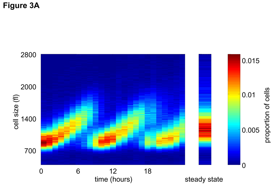
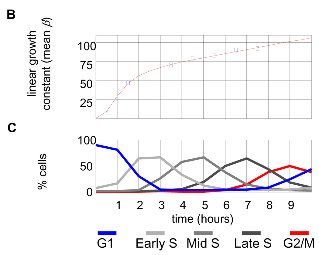
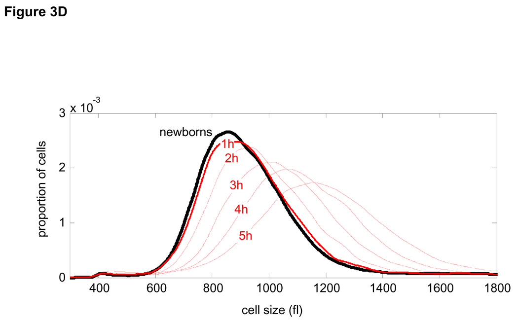
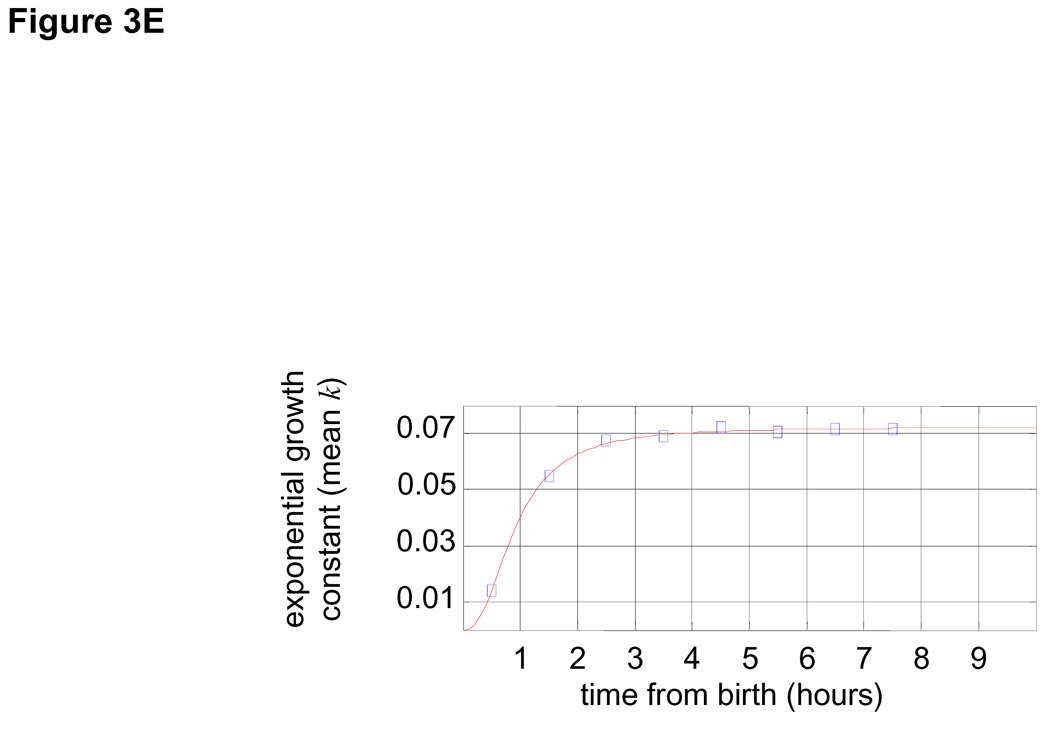
(A) Newborn L1210 cells were incubated at 37°C. Aliquots of cells were taken every hour from zero to 24 hours to measure the size distribution of the synchronous population as it progress through 2.5 cycles. Proportions of cells at any given size are visualized by color (see color bar at the right). Also shown the time-invariant steady-state distribution of the asynchronous population (right panel). (B) The mean linear ,βn , growth constants for each of the time intervals were calculated from Eq. 2 and are expressed in fl/hour. Also shown is the distribution of cell cycle stages (C). (D) Growth repression visualized from raw size distribution measurements. Size distributions of the synchronized L1210 population are shown for early times in cell cycle just after release from the membrane, The size distribution of newborns (black) is compared with distributions from times t=1 hour (red, solid) and times t = 2 – 5 hours (red , dashed). There is very little change from time t = 0 to time t = 1, indicative of the growth repression during the first hour. The larger shifts in the size distribution for later times indicates faster growth later in the cell cycle. (E) The mean exponential, kn, growth constants for each of the time intervals were calculated from Eq. 2 and are expressed in hour−1
(A) Newborn L1210 cells were incubated at 37°C. Aliquots of cells were taken every hour from zero to 24 hours to measure the size distribution of the synchronous population as it progress through 2.5 cycles. Proportions of cells at any given size are visualized by color (see color bar at the right). Also shown the time-invariant steady-state distribution of the asynchronous population (right panel). (B) The mean linear ,βn , growth constants for each of the time intervals were calculated from Eq. 2 and are expressed in fl/hour. Also shown is the distribution of cell cycle stages (C). (D) Growth repression visualized from raw size distribution measurements. Size distributions of the synchronized L1210 population are shown for early times in cell cycle just after release from the membrane, The size distribution of newborns (black) is compared with distributions from times t=1 hour (red, solid) and times t = 2 – 5 hours (red , dashed). There is very little change from time t = 0 to time t = 1, indicative of the growth repression during the first hour. The larger shifts in the size distribution for later times indicates faster growth later in the cell cycle. (E) The mean exponential, kn, growth constants for each of the time intervals were calculated from Eq. 2 and are expressed in hour−1
(A) Newborn L1210 cells were incubated at 37°C. Aliquots of cells were taken every hour from zero to 24 hours to measure the size distribution of the synchronous population as it progress through 2.5 cycles. Proportions of cells at any given size are visualized by color (see color bar at the right). Also shown the time-invariant steady-state distribution of the asynchronous population (right panel). (B) The mean linear ,βn , growth constants for each of the time intervals were calculated from Eq. 2 and are expressed in fl/hour. Also shown is the distribution of cell cycle stages (C). (D) Growth repression visualized from raw size distribution measurements. Size distributions of the synchronized L1210 population are shown for early times in cell cycle just after release from the membrane, The size distribution of newborns (black) is compared with distributions from times t=1 hour (red, solid) and times t = 2 – 5 hours (red , dashed). There is very little change from time t = 0 to time t = 1, indicative of the growth repression during the first hour. The larger shifts in the size distribution for later times indicates faster growth later in the cell cycle. (E) The mean exponential, kn, growth constants for each of the time intervals were calculated from Eq. 2 and are expressed in hour−1
(A) Newborn L1210 cells were incubated at 37°C. Aliquots of cells were taken every hour from zero to 24 hours to measure the size distribution of the synchronous population as it progress through 2.5 cycles. Proportions of cells at any given size are visualized by color (see color bar at the right). Also shown the time-invariant steady-state distribution of the asynchronous population (right panel). (B) The mean linear ,βn , growth constants for each of the time intervals were calculated from Eq. 2 and are expressed in fl/hour. Also shown is the distribution of cell cycle stages (C). (D) Growth repression visualized from raw size distribution measurements. Size distributions of the synchronized L1210 population are shown for early times in cell cycle just after release from the membrane, The size distribution of newborns (black) is compared with distributions from times t=1 hour (red, solid) and times t = 2 – 5 hours (red , dashed). There is very little change from time t = 0 to time t = 1, indicative of the growth repression during the first hour. The larger shifts in the size distribution for later times indicates faster growth later in the cell cycle. (E) The mean exponential, kn, growth constants for each of the time intervals were calculated from Eq. 2 and are expressed in hour−1
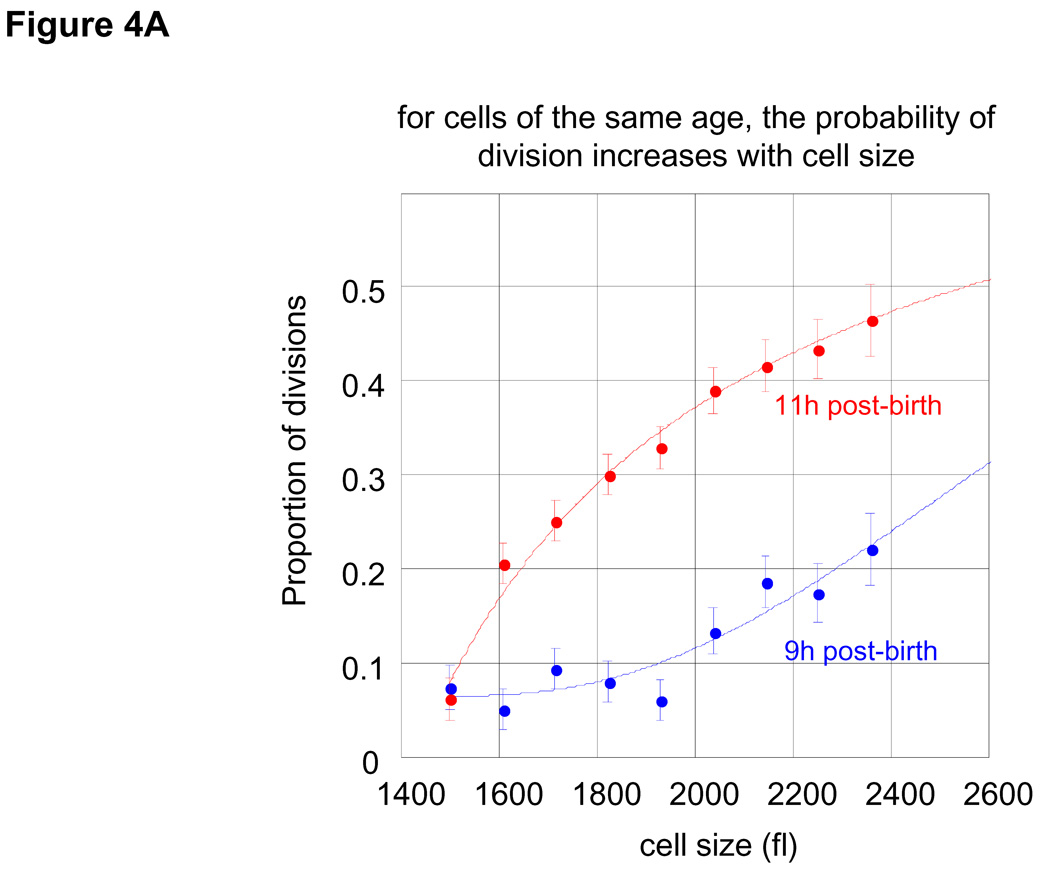
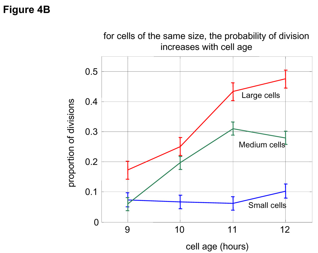
(A) Proportion of cells that have divided at any specified size are shown for cells at 9 hours after birth (blue) and 11 hours after birth (red). For example, it is seen that at 11 hour post-birth about 20% of all cells with size 1600 fl divide. Size distributions were calculated based on a Gaussian kernel. B. Division frequencies as a function of age (each time point represents a one hour interval starting at the indicated times) for cells with size ranging from 1500 to 1850 fl (blue), from 1850 to 2200 fl (green) and from 2250 to 2500 fl (red).
(A) Proportion of cells that have divided at any specified size are shown for cells at 9 hours after birth (blue) and 11 hours after birth (red). For example, it is seen that at 11 hour post-birth about 20% of all cells with size 1600 fl divide. Size distributions were calculated based on a Gaussian kernel. B. Division frequencies as a function of age (each time point represents a one hour interval starting at the indicated times) for cells with size ranging from 1500 to 1850 fl (blue), from 1850 to 2200 fl (green) and from 2250 to 2500 fl (red).
Comment in
-
Cell biology. Sizing up the cell.Science. 2009 Jul 10;325(5937):158-9. doi: 10.1126/science.1177203. Science. 2009. PMID: 19589991 No abstract available.
References
-
- Jorgensen P, Tyers M. Curr Biol. 2004 Dec 14;14:R1014. - PubMed
-
- Mitchison JM. International Review of Cytology. 2003;226:94. - PubMed
-
- Trucco E. Bull Math Biophys. 1970 Dec;32:459. - PubMed
-
- Trucco E, Bell GI. Bull Math Biophys. 1970 Dec;32:475. - PubMed
-
- Tyson JJ, Hannsgen KB. J Math Biol. 1985;22:61. - PubMed
Publication types
MeSH terms
Grants and funding
LinkOut - more resources
Full Text Sources
Other Literature Sources
