Sensitivity Measures for Oscillating Systems: Application to Mammalian Circadian Gene Network

Abstract

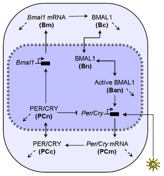
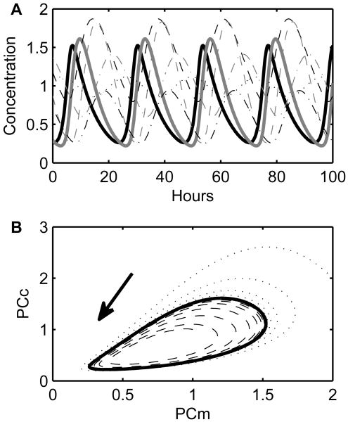
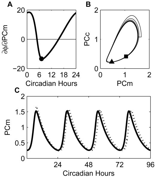
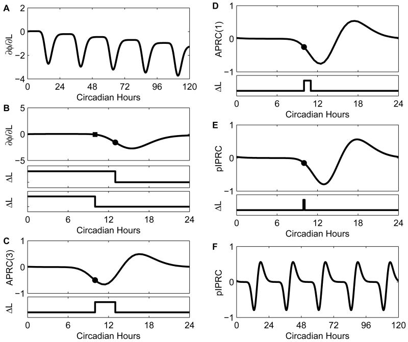
Vital physiological behaviors exhibited daily by bacteria, plants, and animals are governed by endogenous oscillators called circadian clocks. The most salient feature of the circadian clock is its ability to change its internal time (phase) to match that of the external environment. The circadian clock, like many oscillators in nature, is regulated at the cellular level by a complex network of interacting components. As a complementary approach to traditional biological investigation, we utilize mathematical models and systems theoretic tools to elucidate these mechanisms. The models are systems of ordinary differential equations exhibiting stable limit cycle behavior. To study the robustness of circadian phase behavior, we use sensitivity analysis. As the standard set of sensitivity tools are not suitable for the study of phase behavior, we introduce a novel tool, the parametric impulse phase response curve (pIPRC).

Fig. 1

Circadian clock model network. The diagram is adapted from Fig 1 in (Geier et al, 2005). The bold letters denote the states. The solid arrows indicate positive influence. For example, greater concentration (up regulation) of Bmal1 mRNA causes greater concentration of cytoplasmic BMAL1. The flat-headed arrows indicate negative influence. For example, nuclear PER/CRY inhibits the transcription of Per/Cry mRNA . The dashed arrows indicate degradation. There is a negative feedback loop formed by the mRNA and protein versions of Per/Cry. Interlocked with it is a positive feedback loop involving Bmal1 mRNA, BMAL1 protein, and Per/Cry. Light enters the system by modulating the transcription rate of Per/Cry mRNA (PCm). In this study, we use the gating function associated with nocturnal animals.

Fig. 2

Circadian clock model dynamics. (A) A simulation in constant darkness is shown as a function of time. Per/Cry mRNA (PCm) and cytoplasmic PER/CRY (PCc) are shown with the thick lines. (B) The same simulation is shown in phase space (solid line). The dotted and dashed lines represent additional simulations with initial conditions off the periodic orbit (limit cycle). They evolve to the limit cycle, demonstrating that the system has a stable attracting limit cycle.

Fig. 3

Limit cycle with isochrons. The limit cycle is for a 2-state system in which a solution will move around the limit cycle in a counter-clockwise direction. The isochron represented by the dotted line intersects the limit cycle at the peak of state x₁. The isochron represented by the dashed-dotted line intersects the limit cycle at a position encountered 7 hours later, i.e if the first isochron is η(t₁), then this isochron is η(t₁ + 7). Any initial conditions chosen along the same isochron will approach the same position on the limit cycle as time evolves.

Fig. 4

System under a state perturbation. (A) The state IPRC for the state representing Per/Cry mRNA (PCm) shows early morning advances and midday delays. To illustrate its utility we perform a numerical experiment using the prediction of the phase shift due to a perturbation in PCm at CT7.1 (circle). Since ∂φ/∂PCm = −13.351 at CT7.1, we predict that a positive perturbation of 0.15 in PCm at CT7.1 will cause a phase shift Δφ ≈ −13.351 · 0.15 = −2.0027, which means there will be a 2-circadian hour delay. (B) In phase space, we show the concentrations of PCm and cytoplasmic PER/CRY (PCc) to show the limit cycle behavior of the numerical experiment. There is a clear deviation from the limit cycle when the perturbation is introduced. The square marks the position of the unperturbed system at CT293 while the triangle marks the position of the perturbed system at the same time. Since the flow about the limit cycle is counter-clockwise, this indicates the perturbed system is lagging. (C) Here we show the same data, but as a function of time. The concentration of PCm in the perturbed system (dotted line) peaks after that in the unperturbed system (solid line) and we observe a 1.9-circadian hour delay.

Fig. 5

Relationship between parametric phase sensitivity, analytical phase response curves (APRCs), and parametric impulse PRCs (pIPRCs). (A) The parametric phase sensitivity to infinitesimal perturbations in light (L) grows with time. Each point on the phase sensitivity curve can be used to predict the delay or advance that will be incurred due to the release of a sustained perturbation in the parameter L. The overall negative slope indicates that, in general, the longer L remains perturbed, the more delayed the system will be. (B) We show the parametric phase sensitivity over the first period. The values at CT10 (filled square) and CT13 (filled circle) predict the accumulated phase shifts between CT0 and CT10, and between CT0 and CT13, respectively. The corresponding perturbation shapes are illustrated in the lower panels. We observe that the phase changes accumulated between CT10 and CT13 can be predicted by subtracting dφ/dL(13) − dφ/dL(10). (C) The analytical PRC, APRC(t,3), predicts the shift due to a 3-circadian hour pulse. To compute APRC(t,3), we subtract dφ(t + 3)/dL − dφ(t)/dL and divide by 3. The lower panel shows the trace of the L perturbation (the signal) to which the APRC at CT10 predicts the response. (D) APRC(1) is the analytical PRC to a 1-circadian hour pulse. The pulse starting at CT10 is highlighted. As the pulses get shorter in duration, the APRC approaches the slope of the phase sensitivity. (E) The IPRC is the slope of the phase sensitivity and it predicts the phase shift in response to an impulse perturbation - a pulse that is infinitesimal in both duration and magnitude. The prediction associated with an impulse at CT10 is highlighted and the pulse shape is shown in the lower panel. (F) The parametric IPRC is periodic.

Fig. 6

Numerical experimental PRC's. We plot the phase shifts contains the numerical experimental PRC (pluses), pIPRC_L-predicted PRC (solid line), and APRC_L-predicted PRC (dashed line). Each phase shift is plotted for the time at the center of the light pulse. (A) Numerical experimental PRC for 1 Circadian Hour-Pulses of light at 10% strength. For each plus in the numerical experiment, a simulation was performed in which the light parameter L was 0.1 during the light pulse and 0 otherwise. After one week was simulated, we compared the time of the peak in the perturbed system to that of the peak of PCm in the nominal system. The time-step resolution and, therefore, the accuracy of this computation is, at best, 0.01 hour. (B) Numerical experimental PRC for pulse of light at 50% strength. (C) Numerical experimental PRC for pulse of light at 100% strength (L = 1).

Fig. 7

Numerical experimental PRCs. Each plot contains the phase shifts for the numerical experimental PRC (pluses), pIPRC_L-predicted PRC (solid gray line), and APRC_L-predicted PRC (dotted black line). The signal is sinusoidal and its active part lasts 1 hour for the first row, 3 hours for the second row, and 6 hours for the third row. The signal maximum is at 10%, 50%, and 100% of full light, respectively. Notice the different scales on the y-axes.

References

-
- Sontag ED. Some new directions in control theory inspired by systems biology. IET Syst Biol. 2004 Jun;1(no. 1):9–18. [Online]. Available: http://dx.doi.org/10.1049/sb:20045006. - DOI - PubMed
- Kitano H. Systems biology: a brief overview. Proc Natl Acad Sci USA. 2002;295:1662–1664. [Online]. Available: http://dx.doi.org/10.1126/science.1069492. - DOI - PubMed
- Doyle FJ, III, Stelling J. Systems interface biology. J R Soc Interface. 2006 Oct;3(no. 10):603–616. [Online]. Available: http://dx.doi.org/10.1098/rsif.2006.0143. - DOI - PMC - PubMed
- Csete M, Doyle J. Reverse engineering of biological complexity. Proc Natl Acad Sci USA. 2002;295:1664–1669. [Online]. Available: http://dx.doi.org/10.1126/science.1069981. - DOI - PubMed
- Stelling J, Sauer U, Szallasi Z, Doyle FJ, III, Doyle J. Robustness of cellular functions. Cell. 2004 Sep;118(no. 6):675–85. [Online]. Available: http://dx.doi.org/10.1016/j.cell.2004.09.008. - DOI - PubMed
Grants and funding
LinkOut - more resources
Full Text Sources
Research Materials