. 2009 Jul;116(3):519-39.
doi: 10.1037/a0016171.

The behavioral economics of choice and interval timing

Affiliations

The behavioral economics of choice and interval timing

J Jozefowiez et al. Psychol Rev. 2009 Jul.

Abstract

The authors propose a simple behavioral economic model (BEM) describing how reinforcement and interval timing interact. The model assumes a Weber-law-compliant logarithmic representation of time. Associated with each represented time value are the payoffs that have been obtained for each possible response. At a given real time, the response with the highest payoff is emitted. The model accounts for a wide range of data from procedures such as simple bisection, metacognition in animals, economic effects in free-operant psychophysical procedures, and paradoxical choice in double-bisection procedures. Although it assumes logarithmic time representation, it can also account for data from the time-left procedure usually cited in support of linear time representation. It encounters some difficulties in complex free-operant choice procedures, such as concurrent mixed fixed-interval schedules as well as some of the data on double bisection, which may involve additional processes. Overall, BEM provides a theoretical framework for understanding how reinforcement and interval timing work together to determine choice between temporally differentiated reinforcers.


Figures

Figure 1
Figure 1
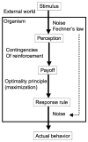
BEM at a glance: (a) based on its perception of the stimulus, the animal emits the behavior which leads to the higher payoff; (b) but its perception is noisy; that is, (c) it follows Fechner’s law; at objective time t, the representation of time is a random variable drown from a Gaussian distribution with a mean equal to ln t and a constant standard deviation.
Figure 2
Figure 2
Conditional probability P(x|t) as a function of x for t = 20 s and t = 60 s. σ = 0.25, ε = 0.001.
Figure 3
Figure 3
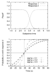
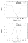
Simulation of a bisection procedure. Response 1 is reinforced after a 20-s stimulus; response 2 after a 60-s stimulus. Top panel: Payoff function for each response in subjective time. Bottom panel: Probability of emitting response 2 as a function of the duration of the test stimulus for various values of σ. The vertical line shows the location of the geometric mean between 20 s and 60 s
Figure 4
Figure 4
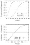
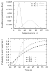
Simulation of timescale invariance in the bisection procedure. Top panel: Probability of emitting response 2 as a function of the test stimulus duration expressed in real time in two bisection tasks. In one task, response 1 is reinforced after a 10-s stimulus, response 2 after a 30-s stimulus. In the other task, response 1 is reinforced after a 20-s stimulus, response 2 after a 60-s one. Bottom panel: same graph but plotted in relative time.
Figure 5
Figure 5
A bisection analogue of the free-operant Bizo and White psychophysical procedure. The animal can emit two responses b1 and b1. Response bi is reinforced at time Ti1 and Ti2 with A amount of reinforcer. The probability of reinforcement of response bi at time Tij is pij. Each stimulus duration Tij has the same probability of occurrence during a session (0.25).
Figure 6
Figure 6
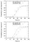
Reinforcement-probability effect on the probability of responding in a bisection analogue of the free-operant psychophysical procedure. Response 1 is reinforced after a stimulus lasting either 10 or 20 s. Response 2 is reinforced after a stimulus lasting either 40 or 80 s. In the control condition, the reinforcement probability for response 1 and response 2 is 0.25. In the “bias b1” condition, the reinforcement probability is 0.75 for response 1 and 0.25 for response 2. In the “bias b2” condition, this is reversed: the reinforcement probability is 0.25 for response 1 and 0.75 for response 2. σ = 0.25.
Figure 7
Figure 7
Reinforcement-probability effect on the payoff functions in a bisection analogue of the free-operant Bizo and White psychophysical procedure. Response 1 is reinforced after a stimulus lasting either 10 or 20 s. Response 2 is reinforced after a stimulus lasting either 40 or 80 s. Top panel: payoff functions in the control condition where the reinforcement probability for each response was 0.25. Bottom panel: payoff function in the “bias b1” condition where the reinforcement probability for response 1 was 0.75 while it was 0.25 for response 2. σ = 0.25.
Figure 8
Figure 8
BEM applied to the Bizo and White data: response 1 is reinforced during the first 25 s according to a VI x while response 2 is reinforced during the last 25 s according to a VI y (the legend shows the value of x/y for each condition). The points are the actual pigeon data while the lines are the predictions of the model. σ was set to 0.3 for all these simulations.
Figure 9
Figure 9
Further effects of probability of reinforcement in a bisection analogue of the free-operant psychophysical procedure. Response 1 is reinforced after a stimulus lasting either 10 or 20 s. Response 2 is reinforced after a stimulus lasting either 40 or 80 s. In the control condition, the reinforcement probability for responses 1 and 2 is 0.25, whatever the stimulus. In condition 1, the probability of reinforcement is 0.75 after a 20-s stimulus for response 1 and after a 80-s stimulus for response 2 while it is 0.25 after a 10-s stimulus for response 1 and after a 40-s stimulus for response 2. In condition 2, the probability of reinforcement is 0.75 after a 10-s stimulus for response 1 and after a 80-s stimulus for response 2 while it is 0.25 after a 20-s stimulus for response 1 and after a 40-s stimulus for response 2. σ = 0.25.
Figure 10
Figure 10
Further effect of probability of reinforcement in a bisection analogue of the free-operant psychophysical procedure. Response 1 is reinforced after a stimulus lasting either 10 or 20 s. Response 2 is reinforced after a stimulus lasting either 40 or 80 s. Top panel: Payoff functions in condition 1. The reinforcement probability for response 1 and response 2 is 0.25, whatever the stimulus. In condition 1, the probability of reinforcement is 0.75 after a 20-s stimulus for response 1 and after a 80-s stimulus for response 2 while it is 0.25 after a 10-s stimulus for response 1 and after a 40-s stimulus for response 2. Bottom panel: Payoff functions in condition 2. The probability of reinforcement is 0.75 after a 10-s stimulus for response 1 and after a 80-s stimulus for response 2 while it is 0.25 after a 20-s stimulus for response 1 and after a 40-s stimulus for response 2. σ = 0.25.
Figure 11
Figure 11
Quantitative fit to the data from Machado and Guilhardi’s (2000) Experiment 1: response 1 is reinforced during the first 30 s of a trial, first according to a VI x then according to a VI x′; response 2 is reinforced for the last 30 s of a trial, first according to a VI y then according to a VI y′ (the legend shows the value of x-x′/y-y′ for each condition). The points are the actual pigeon data while the lines are the predictions of the model. σ a was set to 0.31 for all these simulations.
Figure 12
Figure 12
Quantitative fit to the data from Machado and Guilhardi’s (2000) Experiment 2: response 1 is reinforced during the first 30 s of a trial, first according to a VI x then according to a VI x′; response 2 is reinforced for the last 30 s of a trial, first according to a VI y then according to a VI y′ (the legend shows the value of (x-x′)/(y-y′) for each condition). The points are the actual pigeon data while the lines are the predictions of the model. σ was set to 0.26 for all these simulations.
Figure 13
Figure 13
Payoff function in a double-bisection task. The subjects were submitted to two bisection tasks simultaneously: task 1 pitted a 1-s stimulus versus a 4-s one; task 2 pitted a 4-s stimulus versus a 16-s one. Top panel: Payoff functions for each of the four responses. Bottom panel: Payoff functions for the two responses reinforced after a 4-s stimulus. σ = 0.5.
Figure 14
Figure 14
Double bisection. The subjects were exposed to two bisection tasks simultaneously: task 1 pitted a 1-s stimulus versus a 4-s one; task 2 pitted a 4-s stimulus versus a 16-s one. They were then exposed to a test stimulus whose duration varied between 1 and 16 s and given the choice between the two responses reinforced after a 4-s stimulus: the one from task 1 and the one from task 2. The graph shows the probability of picking the former as a function of the duration of the test stimulus. The points are the pigeons’ data from Machado and Pata (2003). The line is BEM’s predictions. σ = 1.8.
Figure 15
Figure 15
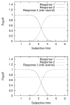
Payoff functions in a “metacognition” task. Response 1 is reinforced with A units of reinforcer after a 10-s or a 20-s stimulus. Response 2 is reinforced with A units of reinforcer after a 40-s or a 80-s stimulus. Response 3 is reinforced with A/2 units of reinforcer, no matter the stimulus duration. A is the objective amount of reinforcer collected. The subjective amount of reward experienced is Ac. Top panel: c = 1, the animal is risk-neutral. Bottom panel: c = 0.5, the animal is risk-averse. σ = 0.5, A = 1.
Figure 16
Figure 16
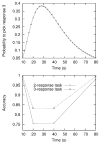
Performance in a “metacognition” task. Response 1 is reinforced with A units of reinforcer after a 10-s or a 20-s stimulus. Response 2 is reinforced with A units of reinforcer after a 40-s or a 80-s stimulus. Response 3 is reinforced with A/2 units of reinforcer, no matter what the stimulus duration. A is the objective amount of reinforcer collected. The subjective amount of reward experienced is Ac. Top panel: Probability of picking response 3 as a function of the stimulus duration. Bottom panel: Accuracy in the 3-response task versus a 2-response task where response 3 is not available. σ = 0.5, c = 0.5.
Figure 17
Figure 17
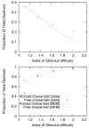
Top panel: Probability of declining a test (that is to say, of selecting the weakly reinforced response) as a function the index of stimulus difficulty used by Foote and Crystal (2007) (this index represents the distance to the boundary between the stimulus classes, thus stimuli on the fringe of the stimulus range, hence easier to discriminate, have a higher index of stimulus difficulty). The points are the data from Foote and Crystal (2007) while the line is the prediction from BEM. Bottom panel: accuracy in the forced choice (2 responses available) and free-choice (3 responses available) trials as a function of the index of stimulus difficulty. The points are the data from Foote and Crystal (2007), the lines are the predictions from BEM. σ = 0.38, c = 0.46.
Figure 18
Figure 18
BEM with a linear representation of time: at time t, the representation is drawn from a Gaussian distribution with a mean t and a standard deviation st. Top panel: Conditional probability P(x|t) as a function of x for t = 20 s and t = 60 s. Bottom panel: Probability of emitting response 2 in a bisection experiment where response 1 was reinforced after a 20-s stimulus and response 2 after a 60-s stimulus for various values of s. The vertical line is the geometric mean between 20 and 60 s.
Figure 19
Figure 19
The time-left procedure. During the initial link, the animal can choose freely between the time-left and the standard side. But T s in a trial (T is determined randomly on each trial according to an arithmetic VI schedule), the procedure moves to the terminal link: the animal’s choice commits it to the schedule it was responding on (the other schedule becomes unavailable). If it is the time-left side, food is available CT s later. If it is the standard side, food is available S s later. Note that a stimulus change takes place when the animal chooses the standard side and moves to the terminal link while no such change occurs in the case of the time-left side.
Figure 20
Figure 20
Simulation of the time-left procedure. The animal can choose between the standard and the time-left side. T s in a trial, it is committed to the side it is responding on: if it is the standard side, reinforcement will occur S later; if it is the time-left side, it will occur CT s later. The graph shows the proportion of responding on the time-left side as a function of time in a trial for various values of S corresponding to the one used by Church and Gibbon (1981). The vertical lines show where the indifference points should be according to the regression line fitted by Church and Gibbon (1981) to their data (0.74S + 1.49). σ = 0.3.
Figure 21
Figure 21
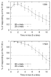
Data from two representative pigeons from Jozefowiez et al. (2005)’s study. The pigeons were exposed to a concurrent FI 20-s FI 60-s. Redrawn from Jozefowiez, J., Cerutti, D.T. and Staddon, J.E.R. (2005), Timing in choice experiments. Journal of Experimental Psychology: Animal Behavior Processes, 31, 213–225.
Figure 22
Figure 22
Proportion of responding on the FI 20-s in a simulation of concurrent FI 20-s FI 60-s for various values of σ.
Figure 23
Figure 23
General procedure in Jozefowiez et al. (2006)’s study. The pigeons had the choice between two mixed FI schedules: one delivering food t1 and t3 s in a trial, the other t2 and t3 s in a trial with t1 < t2 < t3 < t4.
Figure 24
Figure 24
Top panel: Pigeon performance in a concurrent mixed FI 10-s FI 90-s mixed FI 30-s FI 270-s. Redrawn from Jozefowiez, J., Cerutti, D. T. and Staddon, J. E. R. (2006). Timescale invariance and Weber’s law in choice. Journal of Experimental Psychology: Animal Behavior Processes, 32, 229–238. Bottom panel: simulation of the procedure by BEM, for various values of σ. In both figures, the vertical lines show the times of reinforcement (solid and dashed lines) and the geometric means between two successive times of reinforcement (dotted lines).
Figure 25
Figure 25
Top panel: Pigeon performance in a concurrent mixed FI t FI 3t mixed FI 2t FI 4t. t = 10 s in the “short” condition, 20 s in the “medium” condition and 40 s in the “long” condition. Redrawn from Jozefowiez, J., Cerutti, D. T. and Staddon, J. E. R. (2006). Timescale invariance and Weber’s law in choice. Journal of Experimental Psychology: Animal Behavior Processes, 32, 229–238. Bottom panel: Simulation of the “short” condition by BEM for various values of σ. In both figures, the vertical bars show the times of reinforcement.
Figure 26
Figure 26
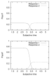
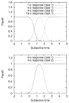
Payoff function in a double-bisection task. The subjects were submitted to two bisection tasks simultaneously: task 1 pitted a 1-s stimulus versus a 4-s one; task 2 pitted a 4-s stimulus versus a 16-s one. The graph shows the payoff functions for the responses associated with the 1-s stimulus (task 1) and the 4-s stimulus (task 2). σ = 0.5.
Figure 27
Figure 27
Payoff functions in the time-left experiment. σ = 0.3, k = 0.9. S = 30 s on the standard side while C = 60 s on the time-left side. Just like in the original Church and Gibbon (1981)’s experiment, transition to the terminal link can take place 5 s in a trial, 10 s, 15 s, etc.

Similar articles

Cited by

References

    1. Ainslie G, Monterosso L. A marketplace in the brain? Science. 2004;306:421–423. - PubMed
    1. Bateson M, Kacelnik K. Preference for fixed and variable food sources: variability in amount and delay. Journal of the Experimental Analysis of Behavior. 1995;63:313–329. - PMC - PubMed
    1. Bizo LA, Chu JYM, Sanabria F, Killeen PR. The failure of Weber’s law in time perception and production. Behavioural Processes. 2006;71:201–210. - PubMed
    1. Bizo LA, White KG. The behavioral theory of timing: reinforcer rate determines pacemaker rate. Journal of the Experimental Analysis of Behavior. 1994a;20:308–321. - PMC - PubMed
    1. Bizo LA, White KG. Pacemaker rate in the behavioral theory of timing. Journal of Experimental Psychology: Animal Behavior Processes. 1994b;20:308–321.

Publication types