A microsaccadic rhythm modulates gamma-band synchronization and behavior

Abstract

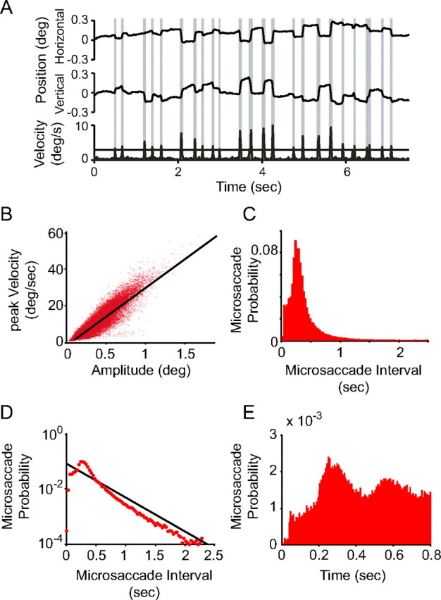
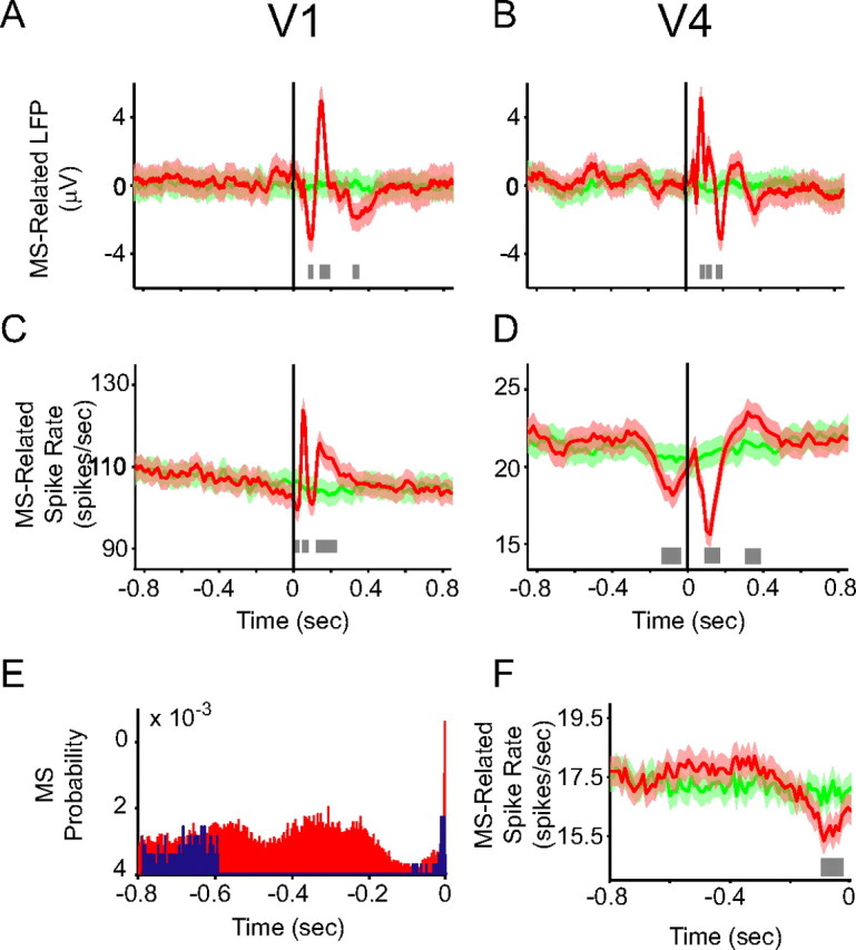
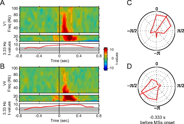
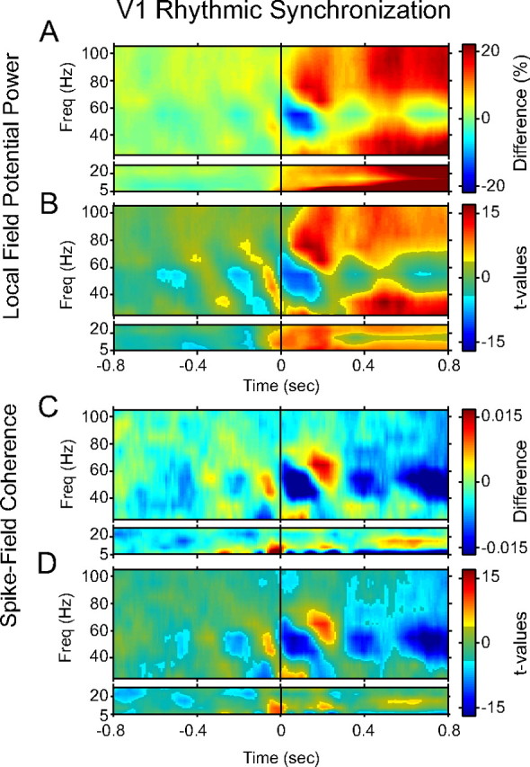
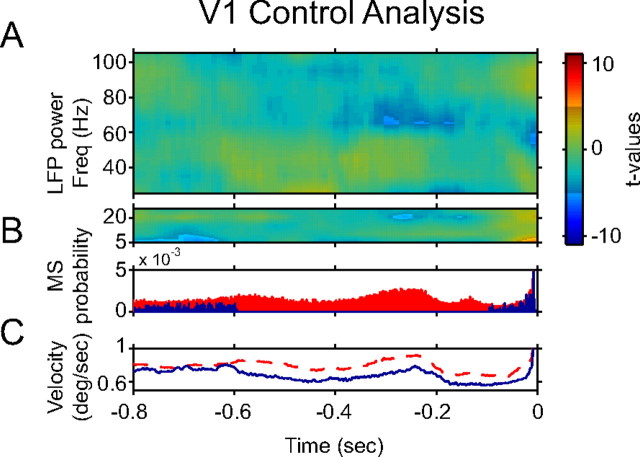
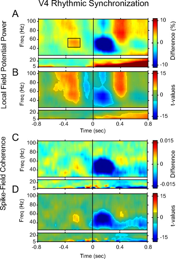
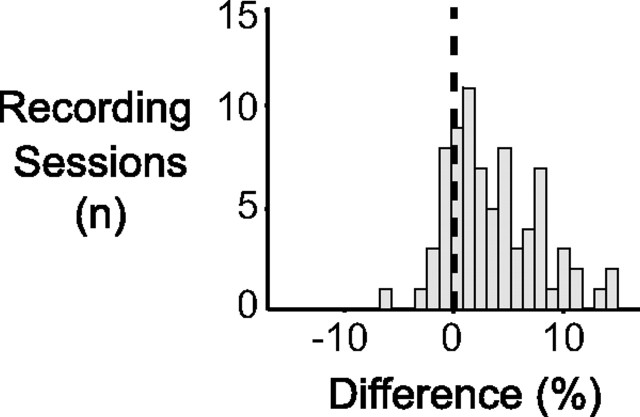
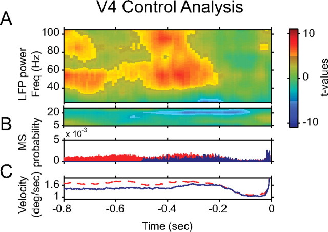
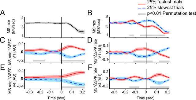
Rhythms occur both in neuronal activity and in behavior. Behavioral rhythms abound at frequencies at or below 10 Hz. Neuronal rhythms cover a very wide frequency range, and the phase of neuronal low-frequency rhythms often rhythmically modulates the strength of higher-frequency rhythms, particularly of gamma-band synchronization (GBS). Here, we study stimulus-induced GBS in awake monkey areas V1 and V4 in relation to a specific form of spontaneous behavior, namely microsaccades (MSs), small fixational eye movements. We found that MSs occur rhythmically at a frequency of approximately 3.3 Hz. The rhythmic MSs were predicted by the phase of the 3.3 Hz rhythm in V1 and V4 local field potentials. In turn, the MSs modulated both visually induced GBS and the speed of visually triggered behavioral responses. Fast/slow responses were preceded by a specific temporal pattern of MSs. These MS patterns induced perturbations in GBS that in turn explained variability in behavioral response speed. We hypothesize that the 3.3 Hz rhythm structures the sampling and exploration of the environment through building and breaking neuronal ensembles synchronized in the gamma-frequency band to process sensory stimuli.

Figure 1.

Microsaccade assessment and statistical characterization. A, Example of eye movement traces and MS detection. Eye position in the horizontal direction (top graph) and vertical direction (middle graph) and the corresponding eye velocity (bottom graph) as a function of time during fixation. The horizontal line in the velocity plot shows the threshold used to detect MSs. Time periods classified as MSs are shaded in gray. B, Scatter plot of MS amplitude versus MS peak velocity (with 1 dot per MS pooled over all MSs used for the neurophysiological analysis), demonstrating the linear relation between both parameters (r = 0.812, p < 0.001, t = 382). C, Histogram (bin width, 0.027 s) of MS probability as a function of time since the last MS. This inter-MS interval histogram shows a peak of MS occurrence at 0.25 s, followed by an exponentially decaying tail. D, Same data as in C, but in semilogarithmic scale to compare with an exponential distribution. The black line illustrates the best-fitting exponential distribution. E, MS autocorrelation histogram (bin width, 0.001 s), directly demonstrating the MS rhythmicity. deg, Degree.

Figure 2.

Microsaccade-related modulations in LFP and spike rate in V1 and V4. A, B, C, D, F, Comparison between MSs related time course averages across sessions (red lines) and fake MSs time course averages across sessions (green lines) (see Materials and Methods for details). Shaded regions around the time courses represent mean ±1 SEM. A, LFP averaged over all trials and recording sites in V1, as a function of time around the MS onset. The bright gray bar at the bottom illustrates significance of the modulation (p < 0.05, randomization test, corrected for multiple comparisons). B, Same as A, but for V4. C, D, Same as A and B, but for spike density function, calculated using Gaussian kernels of 10 ms SD. E, The blue histogram shows the MS autocorrelation function after excluding from the analysis all MSs that were preceded by other MSs within a window of 0.1–0.6 s. The red histogram shows all MSs for comparison. F, The same as D, but after the MS selection as described for E.

Figure 3.

Frequency-wise phase locking of LFP to MSs. A, Top, Time–frequency representation of the inter-MS coherence, expressed as t values for the comparison between MS-aligned and non-MS-aligned LFP segments from V1. Results are shown separately for lower and higher frequency ranges, because different spectral concentrations were used (see Materials and Methods). Bright (gray-masked) colors indicate significance (insignificance) of the respective modulations (p < 0.05, corrected for multiple comparisons across time and frequency). Bottom, Same analysis restricted to the frequency bin of 3.33 ± 1.6 Hz. The gray area indicates the significance threshold. B, Same as A, but for data from V4. C, Polar histogram of V1 LFP phase distributions for 3.33 ± 1.6 Hz and for a 0.6-s-long analysis window centered at 0.333 s before MS onset. D, Same as C, but for data from V4.

Figure 4.

Peri-MS modulation of rhythmic synchronization in V1. A, Time–frequency representation of peri-MS modulations in LFP power as a function of time relative to the MS. Results are shown separately for lower and higher frequency ranges, because different spectral concentrations were used (see Materials and Materials and Methods). B, Time–frequency representation of corresponding t values. Bright (gray-masked) colors indicate significance (insignificance) of the respective modulations (p < 0.05, corrected for multiple comparisons across time and frequency). C, D, Same as A and B, but for spike–field coherence. Freq, Frequency.

Figure 5.

Pre-MS enhancement of V1 gamma-band synchronization is caused by MS rhythmicity. A, Same analysis as for Figure 3B, but after excluding from the analysis all MSs that were preceded by other MSs within a window of 0.1–0.6 s. Freq, Frequency. B, This panel documents the MS selection applied in A and uses only MSs obtained during V1 recordings. The blue histogram shows the MS autocorrelation function after excluding from the analysis all MSs that were preceded by other MSs within a window of −0.6 to −0.1 s. The red histogram shows this autocorrelation function for all MSs. C, The blue line uses the same MSs for the alignment of the analysis as the blue histogram in B, but shows the pre-MS eye velocity. The red line shows the same without MS selection.

Figure 6.

Peri-MS modulation of rhythmic synchronization in V4. A, Time–frequency representation of peri-MS modulations in LFP power as a function of time relative to the MS. Results are shown separately for lower and higher frequency ranges, because different spectral concentrations were used (see Materials and Methods). The black rectangle represents the time–frequency tile used for the analysis shown in Figure 7. B, Time–frequency representation of corresponding t values. Bright (gray-masked) colors indicate significance (insignificance) of the respective modulations (p < 0.05, corrected for multiple comparisons across time and frequency). C, D, Same as A and B, but for spike–field coherence. Freq, Frequency.

Figure 7.

Consistency of pre-MS enhancement of gamma-band synchronization. Histogram of relative change in LFP power across all recording sites for the time–frequency tile indicated in Figure 6A (comparing peri-MS periods with periods not aligned to MSs, as explained in Materials and Methods).

Figure 8.

Pre-MS enhancement of V4 gamma-band synchronization is not caused by MS rhythmicity. A, Same analysis as for Figure 4, but for data from V4 after excluding from the analysis all MSs that were preceded by other MSs within a window of −1.0 to −0.5 s. Freq, Frequency. B, This panel documents the MS selection applied in A and uses only MSs obtained during V4 recordings. The blue histogram shows the MS autocorrelation function after excluding from the analysis all MSs that were preceded by other MSs within a window of 0.5–1.0 s. The red histogram shows this autocorrelation function for all MSs. C, The blue line uses the same MSs for the alignment of the analysis as the blue histogram in B but shows the pre-MS eye velocity. The red line shows the same without MS selection. deg, Degree.

Figure 9.

The efficiency of visuomotor transformation is modulated by the MS rhythm and the corresponding modulations in GBS and spike activity. A, MS rate as a function of time around stimulus change. MS rate was calculated using a sliding window of ±0.05 s. Shaded region around the time course represents mean ± 95% confidence interval. B, MS rate comparison for trials from the fastest (red) and slowest (blue) reaction time quartiles. Bright gray bar at the bottom highlights the significant differences (p < 0.01, nonparametric permutation test). C, Convolution of MS rate time courses as in B with the gamma-band modulation in area V1 (Fig. 4C, gamma-band SFC difference as shown). D, Convolution of MS rate time courses as in B with spike rate modulation in area V1 (difference between normalized spike rates around MSs compared with equivalent epochs without MSs). E, Same as C but for data from V4. F, Same as D but for data from V4.

References

1. Ahissar E, Arieli A. Figuring space by time. Neuron. 2001;32:185–201. - PubMed
1. Bair W, O'Keefe LP. The influence of fixational eye movements on the response of neurons in area MT of the macaque. Vis Neurosci. 1998;15:779–786. - PubMed
1. Bauer M, Oostenveld R, Peeters M, Fries P. Tactile spatial attention enhances gamma-band activity in somatosensory cortex and reduces low-frequency activity in parieto-occipital areas. J Neurosci. 2006;26:490–501. - PMC - PubMed
1. Beeler GW., Jr Visual threshold changes resulting from spontaneous saccadic eye movements. Vision Res. 1967;7:769–775. - PubMed
1. Bichot NP, Rossi AF, Desimone R. Parallel and serial neural mechanisms for visual search in macaque area V4. Science. 2005;308:529–534. - PubMed
Publication types
LinkOut - more resources