Automated voxel-based 3D cortical thickness measurement in a combined Lagrangian-Eulerian PDE approach using partial volume maps

Abstract

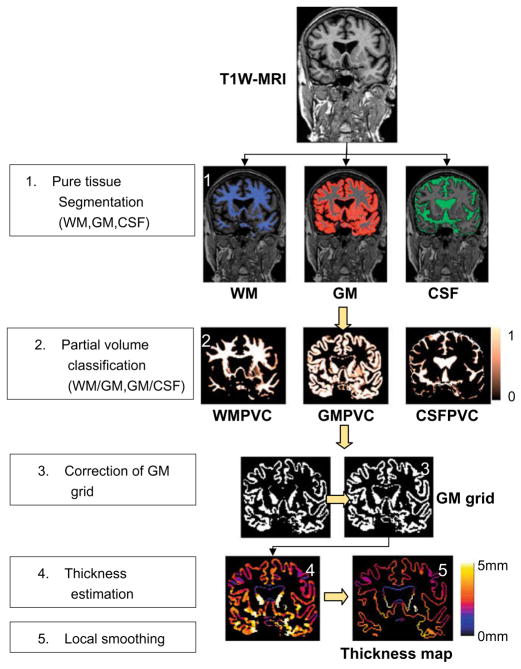
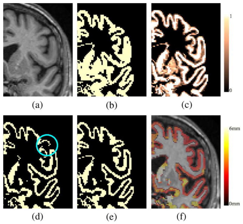
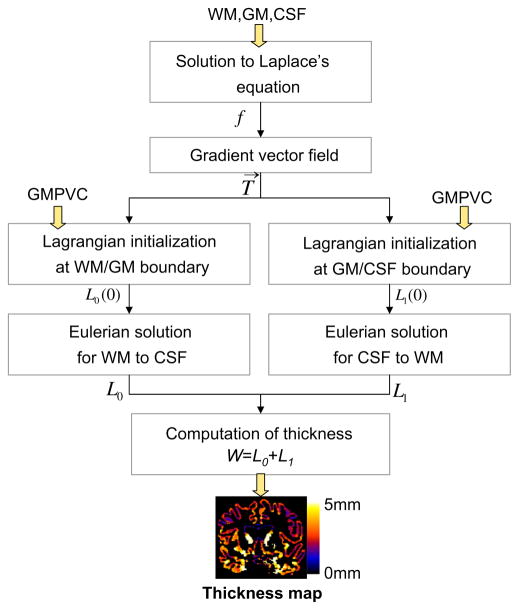
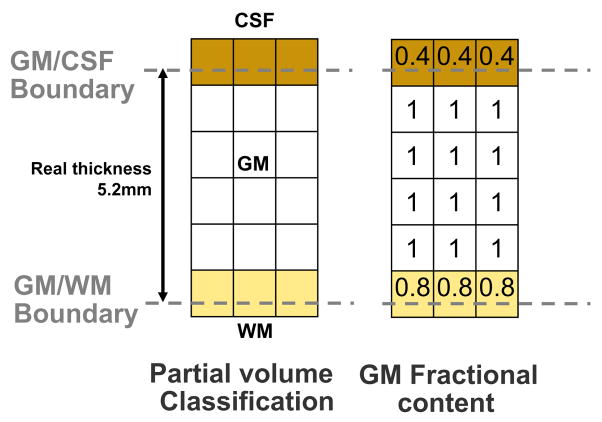
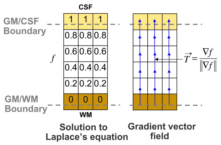
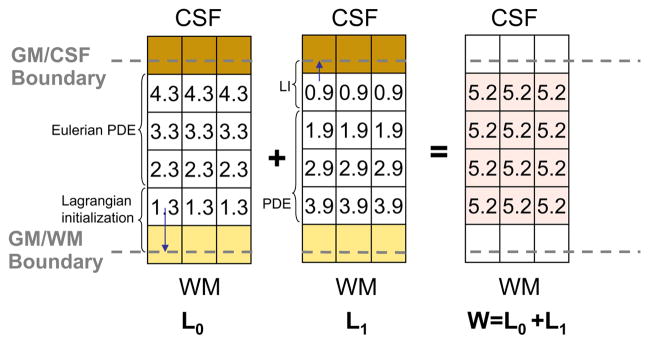
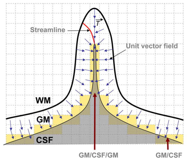
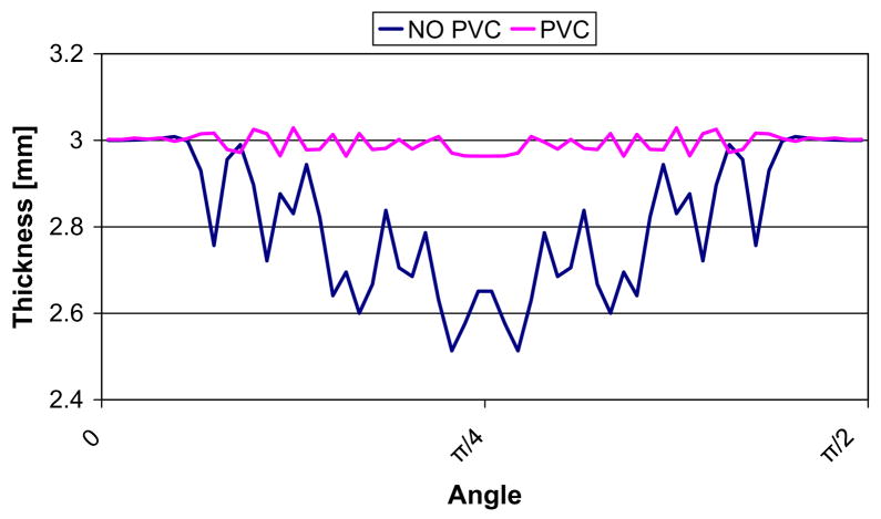
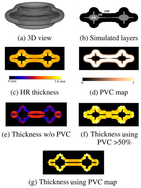
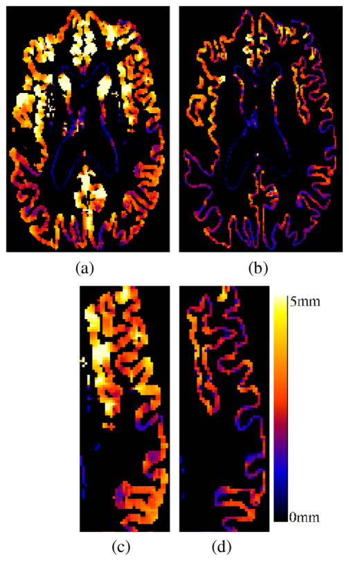
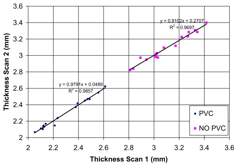
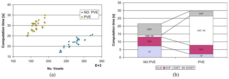
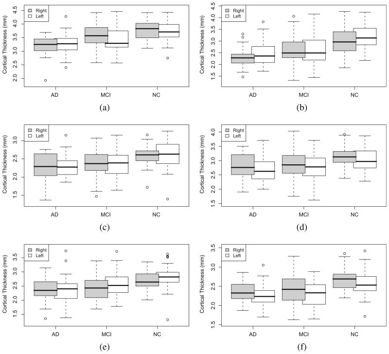
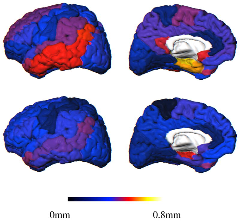
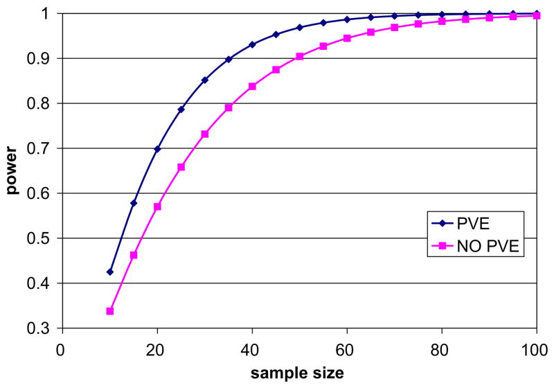
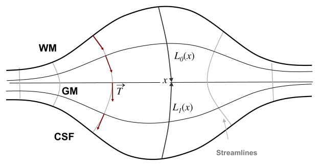
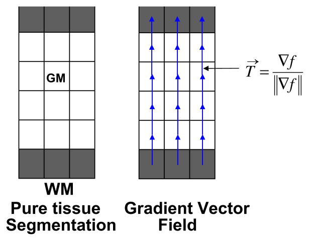
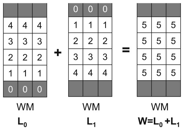
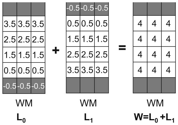
Accurate cortical thickness estimation is important for the study of many neurodegenerative diseases. Many approaches have been previously proposed, which can be broadly categorised as mesh-based and voxel-based. While the mesh-based approaches can potentially achieve subvoxel resolution, they usually lack the computational efficiency needed for clinical applications and large database studies. In contrast, voxel-based approaches, are computationally efficient, but lack accuracy. The aim of this paper is to propose a novel voxel-based method based upon the Laplacian definition of thickness that is both accurate and computationally efficient. A framework was developed to estimate and integrate the partial volume information within the thickness estimation process. Firstly, in a Lagrangian step, the boundaries are initialized using the partial volume information. Subsequently, in an Eulerian step, a pair of partial differential equations are solved on the remaining voxels to finally compute the thickness. Using partial volume information significantly improved the accuracy of the thickness estimation on synthetic phantoms, and improved reproducibility on real data. Significant differences in the hippocampus and temporal lobe between healthy controls (NC), mild cognitive impaired (MCI) and Alzheimer's disease (AD) patients were found on clinical data from the ADNI database. We compared our method in terms of precision, computational speed and statistical power against the Eulerian approach. With a slight increase in computation time, accuracy and precision were greatly improved. Power analysis demonstrated the ability of our method to yield statistically significant results when comparing AD and NC. Overall, with our method the number of samples is reduced by 25% to find significant differences between the two groups.

Fig. 1

Overall process for cortical thickness estimation.

Fig. 2

(a) MR T1W image. (b) Initial GM hard segmentation from EMS. (c) Computed GMPVC map. (d) GM pure tissue voxels (GMPVC = 1). The lost of continuity in the GM is highlighted. (e) Continuity corrected GM grid. (f) Overlaid of resulting thickness map and original MR image.

Fig. 3

Combined Lagrangian–Eulerian thickness estimation.

Fig. 4

Unidimensional model of a voxel occupied by two pure tissues A and B. Top: Voxel i − 1 contains only tissue A, voxel i contains both A and B and voxel i + 1 contains only tissue B. Bottom: PVC representation for the tissue A. The boundary (x₀) of A is found by linear interpolation at APVC = 0.5.

Fig. 5

Example of an isotropic 5.2 voxels thick structure (GM), represented in pure and mixed tissue voxels. If only pure tissue voxels were considered the resulting thickness would be 4.

Fig. 6

Solution to Laplace’s equation and computation of gradient vector field within the GM grid.

Fig. 7

Computation of thickness. After initialization of distance functions L₀ in the GM/WM interface, and L₁ in the GM/CSF interface with the GM fractional content, the PDEs are solved for the remaining voxels. The thickness is computed as expected and the values are updated only in the GM grid.

Fig. 8

Depending on the computed GMPVC for a given GM voxel x, two cases of boundary detection are considered. When GMPVC > 0.5 the ray r follows the direction of the unit vector field. The opposite when GMPVC < 0.5 as the boundary has to be supposed inwards with respect to the centre of the voxel x.

Fig. 9

Partial volumed voxels in deep sulci are composed of a mixture GM/CSF/GM (GM in opposite directions) which can be reapportioned in mixtures GM/CSF and CSF/GM.

Fig. 10

Example of cortical smoothing. (a) Computed cortical thickness map. (b) Smooth map of GM/WM surface using a 5 mm radius sphere over the connected components. (c and d) Marching cubes rendering of voxel maps (a) and (b), respectively.

Fig. 11

Example of partial volume classification on simulated MR data: (a) Initial MR T1 weighted Image (noise 3%, bias field 20%), (b) Hard GM segmentation obtained with EMS algorithm, (c) Ground truth PV map, and (d) Computed GMPVC map.

Fig. 12

Example of thickness computation for a 3 mm synthetic hollow sphere (isotropic 0.5 mm spacing). (a and b) PVC map generated from a high resolution sphere. (c) Computed thickness with initialization at negative half of the voxel spacing. (d) Computed thickness with PVC initialization.

Fig. 13

Comparison of computed thickness for the 0.5 × 0.5 × 0.5 mm sphere. The thickness was measured around the WM/GM surface in the central slice, with angles ranging between 0 and π/2.

Fig. 14

Thickness computation for the spiky phantom. (a) Semitransparent 3D view. (b) 2D cutplane of simulated WM, GM and CSF layers. (c) Pseudo ground truth: computed thickness at high resolution (HR). (d) PVC map generated by subsampling the original phantom by a factor of 8. Computed low resolution thickness maps (e) without using the PVC (only pure tissue voxels), (f) thickness using the PVC > 50%, (g) thickness using PVC map.

Fig. 15

Cortical thickness maps (a and c) without using PVE and (b and d) with the proposed approach. A natural delineation of the sulci is achieved by taking into account the partial volume effect.

Fig. 16

Comparison of mean cortical thickness of the 17 subjects computed from two different scans and with the two methods: (i) No PVE as in Yezzi’s approach and (ii) proposed method using the PV.

Fig. 17

Comparison in computation time, for the cortical thickness estimation part, between the two approaches on real MR data: Eulerian (NO PVE) and Combined Lagrangian–Eulerian (PVE). (a) GM grid size vs. total time. (b) Disaggregated times for each one of the steps. LE: SOR computation of Laplace’s Equation, GVF: Computation of Gradient Vector Field, DIST INI: Initalization of PDEs at the boundaries (Lagrangian in PVE case), DIST: computation time for distances functions L₀ and L₁. When the PV is being used, most of the computation time is spent in the Lagrangian initialization, however this time is compensated by the reduced number of voxels being included in the grid for the Eulerian part.

Fig. 18

Difference in thickness among the three groups for different regions. (a) Parahippocampal gyrus (PHG),(b) hippocampus (Hipp), (c) supramarginal gyrus (SMG), (d) middle temporal gyrus (MTL), (e) angular gyrus, and (f) superior temporal gyrus (STG).

Fig. 19

AAL template showing the regional mean cortical thickness difference between the groups over the surface. Top: NC and AD; Bottom: NC and MCI. Left: lateral and Right: medial views.

Fig. 20

Power analysis for the whole brain: Comparison of power (1 − β) against the number of subjects required using both methods. One can see that using the PVE, a fewer number of subjects is needed when taking partial volume into account to reach high power (>0.8) and detect significant changes between NC and AD.

Fig. A.1

Distance equations L₀ and L₁ for computation of thickness W at a given point x. Thus, W(x) = L₀(x) + L₁(x).

Fig. A.2

Representation of initial pure tissue segmentations (WM, GM and CSF) and computation of the normalised gradient vector field.

Fig. A.3

Since the distances are measured from the centre of the voxels, the initialization of the boundaries at 0 as in Yezzi and Prince (2003) leads to an overestimation of the thickness W= L₀ + L₁.

Fig. A.4

Initialization according to Diep et al. (2007).

References

1. Besag J. On the statistical analysis of dirty pictures. Journal of the Royal Statistical Society. 1986;48:259–302.
1. Collins D, Zijdenbos A, Kollokian V, Sled J, Kabani N, Holmes C, Evans A. Design and construction of a realistic digital brain phantom. IEEE Transactions on Medical Imaging. 1998;17 (3):463–468. - PubMed
1. Dale A, Fischl B, Sereno M. Cortical surface-based analysis I: segmentation and surface reconstruction. NeuroImage. 1999;9 (2):179–194. - PubMed
1. Diep T-M, Bourgeat P, Ourselin S. Efficient use of cerebral cortical thickness to correct brain MR segmentation. IEEE International Symposium on Biomedical Imaging (ISBI’07). IEEE; Washington, DC, USA. 2007. pp. 592–595.
1. Faul F, Erdfelder E, Lang AG, Buchner A. G* power 3: a flexible statistical power analysis program for the social, behavioral, and biomedical sciences. Behavior Research Methods. 2007;39 (2):175–191. - PubMed
Publication types