The viscoelastic properties of passive eye muscle in primates. II: testing the quasi-linear theory

Abstract

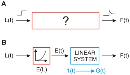
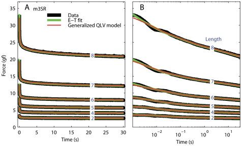
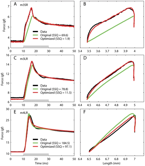
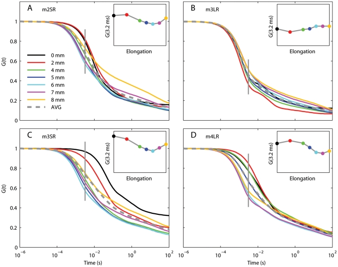
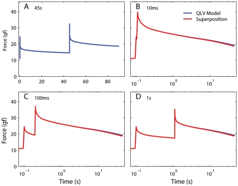
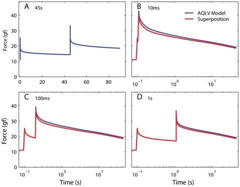
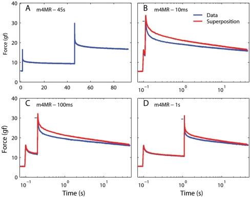
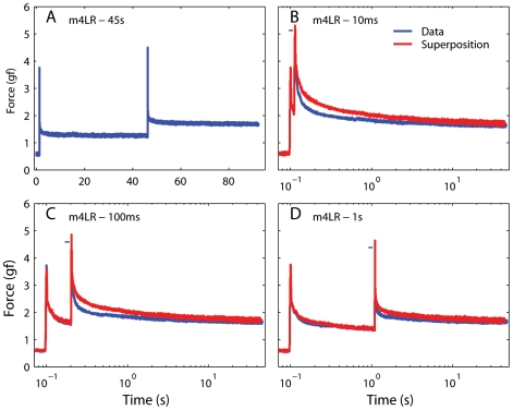
We have extensively investigated the mechanical properties of passive eye muscles, in vivo, in anesthetized and paralyzed monkeys. The complexity inherent in rheological measurements makes it desirable to present the results in terms of a mathematical model. Because Fung's quasi-linear viscoelastic (QLV) model has been particularly successful in capturing the viscoelastic properties of passive biological tissues, here we analyze this dataset within the framework of Fung's theory.We found that the basic properties assumed under the QLV theory (separability and superposition) are not typical of passive eye muscles. We show that some recent extensions of Fung's model can deal successfully with the lack of separability, but fail to reproduce the deviation from superposition.While appealing for their elegance, the QLV model and its descendants are not able to capture the complex mechanical properties of passive eye muscles. In particular, our measurements suggest that in a passive extraocular muscle the force does not depend on the entire length history, but to a great extent is only a function of the last elongation to which it has been subjected. It is currently unknown whether other passive biological tissues behave similarly.

Figure 1. Schematic view of Fung's theory.

A: In most biological passive materials, a stepwise change in elongation (gray trace on the left) causes the force to suddenly increase and then decay over time (gray trace on the right). B: Fung proposed that this response scales with the size of the step, and that there is a nonlinear relationship E(L) between the peak force and the step size (which he called elastic response). He also posited that the decaying response is generated by a linear system, which can be described in terms of its step response. G(t) is then the response of the linear subsystem to a unitary step, 1(t), of the elastic response. This is a cascade of a static nonlinearity and a linear system, often referred to as a Hammerstein system. The model is not limited to reproducing the response to a strain step, but can be used to predict the response to an arbitrary strain history. Blue blocks indicate linear processes, whereas red blocks indicate the presence of a nonlinearity.

Figure 2. Relaxation responses and generalized QLV model fits.

A: Data (black), Emri-Tschoegl fit to the relaxation response (green), and force predicted by the generalized QLV model using the parameters derived analytically from the E-T fit (red). Six different steps are shown (blue numbers are the final lengths in mm), from the superior rectus in m3. B: Same as A, but using a logarithmically spaced abscissa to improve visualization of the force at short times.

Figure 3. Peri-elongation forces and generalized QLV model fits.

Data (black), force predicted by the generalized QLV model using the parameters derived analytically from the E-T fit (green), and force predicted by the generalized QLV model after parameter optimization and addition of a viscous term (red). A: Data for a step at short elongations from the superior rectus in m3. B: Same forces as in A, but plotted as a function of muscle elongation rather than time. The initial rapid rise in force is due to the pure viscosity, which was not part of the original model (green trace). C & D: Same as A & B, but for a step at intermediate elongations from the lateral rectus in m3. E & F: Same as A & B, but for a step at large elongations from the lateral rectus in m4. Note how in this case the fit is not as good, as the force in panel F is convex, whereas the model predictions are always concave. Force scale is different across rows. SSQ: sum of squared residuals (fit – data).

Figure 4. Reduced relaxation function for the generalized QLV model.

In each panel we plot, as a function of time, the step response of the linear part of the QLV model (Fig. 1B). Since we used the generalized QLV model there is a curve for each muscle length. If the separability hypothesis held, these curves should all be identical. In the insets we plot the value of the reduced relaxation function at time 3.2 ms (vertical gray line in the main plots) as a function of elongation. Notice how this relationship is in all cases smooth, which would not be expected if the variations were due to random noise or fitting errors. The label in each panel indicates which monkey (m2, m3 or m4) and muscle (LR = lateral rectus, SR = superior rectus) the data are from. AVG: average reduced relaxation function (gray dashed line).

Figure 5. Schematic view of the adaptive QLV model (Eq. 17).

Blue is used for linear processes, and red is used to indicate nonlinearities. Because the nonlinearity does not precede the linear stage (L.S.), superposition does not hold (unlike the QLV model, Fig. 1B).

Figure 6. Step responses and AQLV model fits.

Data (black) and force predicted by the AQLV model (green). The values for the parameters of the model at each step length were derived from the parameters of the generalized QLV model described above. A cubic spline interpolation (Fig. 7C) was then used to determine the value of the parameters at other lengths. Data for the superior rectus in m3. Each step has been offset in time for clarity. Note that in a logarithmic plot to carry out this operation without deforming the shape the time axis must be compressed, not shifted.

Figure 7. Parameters for the AQLV model.

Each panel shows the parameters for a different muscle, as a function of length at the end of the step. The parameter values (dots) have been computed from the optimized QLV parameters, and the length shown is the muscle length after the end of the step. To estimate the values for an arbitrary length we then either used a cubic spline interpolation (dotted lines, used in Fig. 6), or a four-parameter nonlinear fit (solid lines, used in Fig. 8).

Figure 8. Step responses and AQLV model fits.

Data (black) and force predicted by the AQLV model. A four-parameter non-linear equation was used to fit the values for the parameters derived from the QLV model at each step length (red trace). Because this model has fewer degrees of freedom than the cubic spline used in Fig. 6(and shown here in green), the fit is not as good (gray arrows point to the largest discrepancies between the two models), but it is very good nonetheless. Data for the lateral rectus in m3, the muscle for which we obtained the worst fit between model and data. Just as in Fig. 6, the traces are offset in time for clarity.

Figure 9. The QLV model obeys superposition.

A: A sequence of two elongation steps (0.5 mm each), separated in time by 45 s, was simulated using the generalized QLV model, and the resulting force is plotted against time. B: The same two steps shown in A are applied, but now the temporal separation (ISI) is only 10 ms. (Blue: Model output. Red: Output expected if the superposition principle is obeyed. Note logarithmic scale for time.) C: Same as in B, but with an ISI of 100 ms. D: Same as in C, but with an ISI of 1 s. In all cases the model output matches the superposition prediction. The small deviation between the two traces toward the end of each simulation is due to the incomplete settling of the model output just before the second step in panel A (on which the superposition prediction is based).

Figure 10. The AQLV model does not obey superposition.

Same as Fig. 9, but now the AQLV model is used for the simulations. In all cases the model output is larger than the superposition prediction. The deviation between the two traces is maximal at the end of the second step, and is larger for shorter inter-step intervals. Some of the deviation toward the end of each simulation can be imputed to the incomplete settling of the model output just before the second step in panel A, but the initial deviation is due to the lack of superposition in this model.

Figure 11. Testing the superposition hypothesis in muscle at long lengths.

A: A sequence of two elongation steps (0.5 mm each), separated in time (ISI) by 45 s, was applied, and the resulting force measured. B: The same two steps shown in A are applied, but now the ISI is only 10 ms. (Blue: Force measured. Red: Force predicted by the superposition principle) C: Same as in B, but with an ISI of 100 ms. D: Same as in C, but with an ISI of 1 s. For clarity, the maximum force recorded is marked by a small horizontal blue bar just to the left of the value. In all cases the prediction is initially considerably higher than the actual force, indicating that the superposition principle does not hold in muscle at long lengths.

Figure 12. Testing the superposition hypothesis in muscle at short lengths.

Same as Fig. 11, but in a different muscle and at the low end of the elongation range (notice the much smaller forces). Superposition does not hold at short lengths either.

Figure 13. Force induced by the second step in a double-step sequence.

A: Data from elongations at long lengths, same dataset as in Fig. 11 . The force induced by the second elongation step is not a function of the ISI. B: Data from elongations at short lengths, same dataset as in Fig. 12. With the exception of the first 20 ms after the shortest ISI, the force induced by the second elongation step is invariant. The muscle thus appears to have no memory of the previous elongation.

References

1. Buchthal F, Kaiser E. The rheology of the cross striated muscle fiber, with particular reference to isotonic conditions. Dan Biol Medd. 1951;21:1–318.
1. Bagni MA, Cecchi G, Colombini B, Colomo F. Mechanical properties of frog muscle fibres at rest and during twitch contraction. J Electromyogr Kinesiol. 1999;9:77–86. - PubMed
1. Bagni MA, Cecchi G, Colomo F, Garzella P. Are weakly binding bridges present in resting intact muscle fibers?. Biophys J. 1992;63:1412–5. - PMC - PubMed
1. Bagni MA, Cecchi G, Colomo F, Garzella P. Absence of mechanical evidence for attached weakly binding cross-bridges in frog relaxed muscle fibres. J Physiol. 1995;482:391–400. - PMC - PubMed
1. Mutungi G, Ranatunga KW. The visco-elasticity of resting intact mammalian (rat) fast muscle fibres. J Muscle Res Cell Motil. 1996;17:357–364. - PubMed
Publication types