

Resolving deconvolution ambiguity in gene alternative splicing
- PMID: 19653895
- PMCID: PMC2739860
- DOI: 10.1186/1471-2105-10-237
Resolving deconvolution ambiguity in gene alternative splicing
Abstract
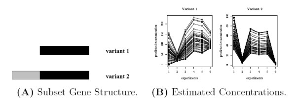
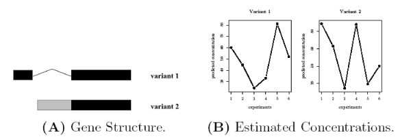
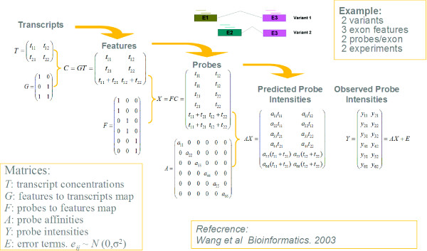
Background: For many gene structures it is impossible to resolve intensity data uniquely to establish abundances of splice variants. This was empirically noted by Wang et al. in which it was called a "degeneracy problem". The ambiguity results from an ill-posed problem where additional information is needed in order to obtain an unique answer in splice variant deconvolution.
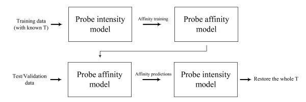
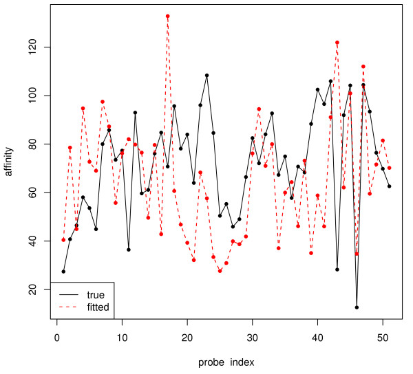
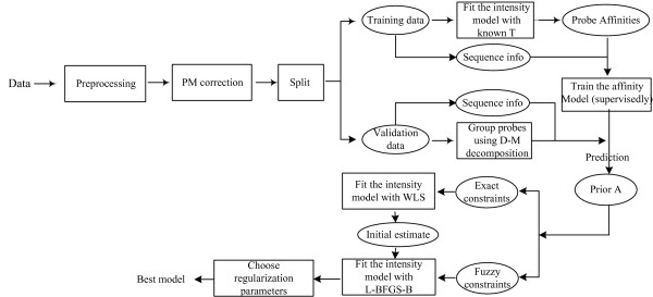
Results: In this paper, we analyze the situations under which the problem occurs and perform a rigorous mathematical study which gives necessary and sufficient conditions on how many and what type of constraints are needed to resolve all ambiguity. This analysis is generally applicable to matrix models of splice variants. We explore the proposal that probe sequence information may provide sufficient additional constraints to resolve real-world instances. However, probe behavior cannot be predicted with sufficient accuracy by any existing probe sequence model, and so we present a Bayesian framework for estimating variant abundances by incorporating the prediction uncertainty from the micro-model of probe responsiveness into the macro-model of probe intensities.
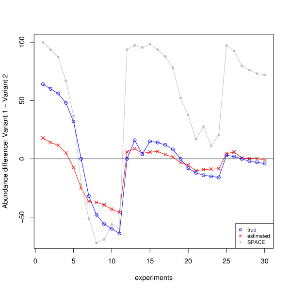
Conclusion: The matrix analysis of constraints provides a tool for detecting real-world instances in which additional constraints may be necessary to resolve splice variants. While purely mathematical constraints can be stated without error, real-world constraints may themselves be poorly resolved. Our Bayesian framework provides a generic solution to the problem of uniquely estimating transcript abundances given additional constraints that themselves may be uncertain, such as regression fit to probe sequence models. We demonstrate the efficacy of it by extensive simulations as well as various biological data.
Figures
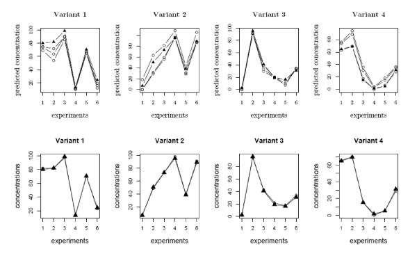
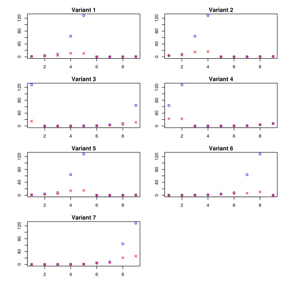
 and the true T.
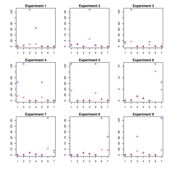 and the true T.
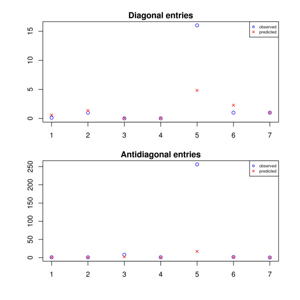 and the true T.
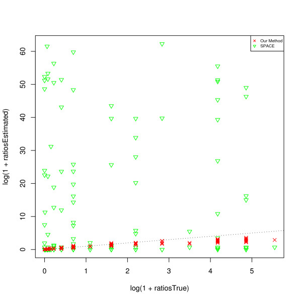
References
Publication types
MeSH terms
LinkOut - more resources
Full Text Sources
