The location of the inferior and superior temporal blood vessels and interindividual variability of the retinal nerve fiber layer thickness

Abstract

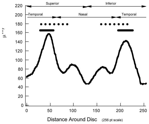
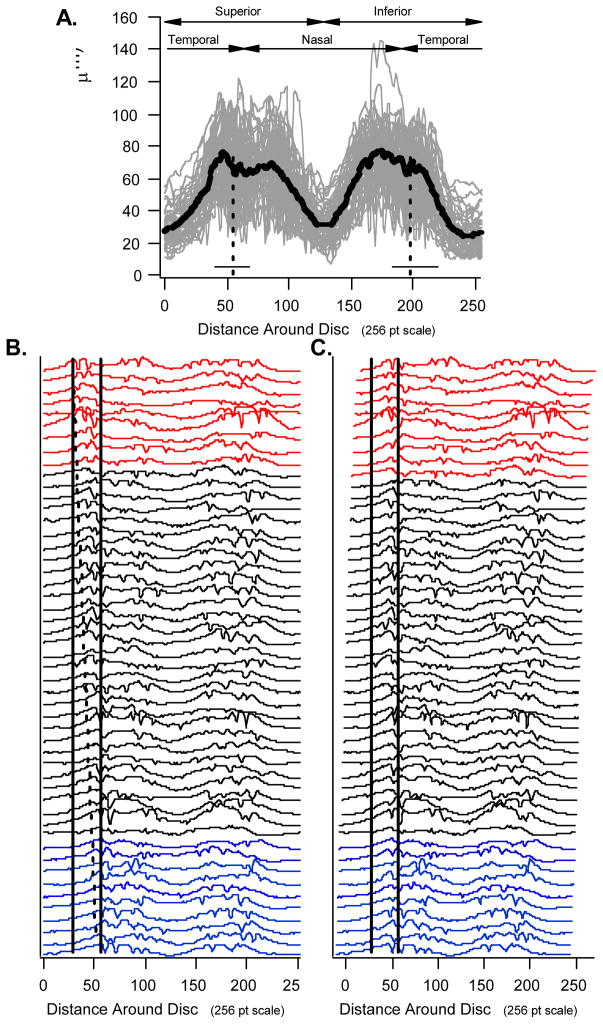
Purpose: To determine if adjusting for blood vessel (BV) location can decrease the intersubject variability of retinal nerve fiber layer (RNFL) thickness measured with optical coherence tomography (OCT).

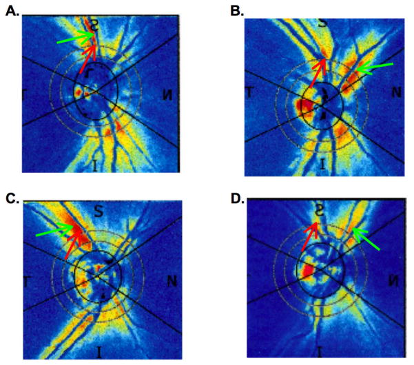
Subjects and methods: One eye of 50 individuals with normal vision was tested with OCT and scanning laser polarimetry (SLP). The SLP and OCT RNFL thickness profiles were determined for a peripapillary circle 3.4 mm in diameter. The midpoints between the superior temporal vein and artery (STva) and the inferior temporal vein and artery (ITva) were determined at the location where the vessels cross the 3.4 mm circle. The average OCT and SLP RNFL thicknesses for quadrants and arcuate sectors of the lower and upper optic disc were obtained before and after adjusting for BV location. This adjustment was carried out by shifting the RNFL profiles based upon the locations of the STva and ITva relative to the mean locations of all 50 individuals.

Results: Blood vessel locations ranged over 39 (STva) and 33 degrees (ITva) for the 50 eyes. The location of the leading edge of the OCT and SLP profiles was correlated with the location of the BVs for both the superior [r=0.72 (OCT) and 0.72 (SLP)] and inferior [r=0.34 and 0.43] temporal vessels. However, the variability in the OCT and SLP thickness measurements showed little change due to shifting. After shifting, the difference in the coefficient of variation ranged from -2.1% (shifted less variable) to +1.7% (unshifted less variable).

Conclusions: The shape of the OCT and SLP RNFL profiles varied systematically with the location of the superior and inferior superior veins and arteries. However, adjusting for the location of these major temporal BVs did not decrease the variability for measures of OCT or SLP RNFL thickness.

FIGURE 1

A. An OCT RNFL thickness profile from a healthy eye. B. Example of a SLP density plot used to export data for SLP analysis. C. SLP RNFL profile obtained around green ring in panel B. D. A fundus image from the SLP report used to identify the location of the major temporal vein and artery in the superior (STva) and inferior (ITva) disc regions. The red and blue lines show the location of STva and ITva and the black arcs show the range of locations for the individuals in this study.

FIGURE 2

The black dashed and solid horizontal lines indicate the regions included within the quadrant and Garway-Heath et al(G-H) sectors, respectively. The curves represent the average OCT RNFL profiles for all 50 eyes.

FIGURE 3

A. The OCT RNFL profiles for all 50 individuals with the mean of these profiles shown in bold. The vertical dashed lines are the mean locations for the STva and ITva and the horizontal solid lines the range. B. The profiles from panel A positioned from top to bottom in order of the location of the STva. C. The same profiles as in panel B, but shifted by an amount equal to the relative locations of the STva.

FIGURE 4

A. The averages of the OCT RNFL profiles in Fig. 3B with the most temporal STva (red) and most nasal STva (blue) along with the mean locations (vertical lines) of the STva for these individuals. B. Same as in panel A, but for an analogous analysis for the ITva and the inferior disc region. C. Same as in panel A, but for the SLP profiles in Fig. 5B. D. Same as in panel C, but for an analogous analysis for the ITva and the inferior disc region.

FIGURE 5

A. The SLP RNFL profiles for all 50 eyes with the mean of these profiles shown in bold. The vertical dashed lines are the mean locations for the STva and ITva and the horizontal solid lines the range. B. The profiles from panel A positioned from top to bottom in order of the location of the STva. C. The same profiles as in panel B, but shifted by an amount equal to the relative locations of the STva.

FIGURE 6

A. Method for determining the location of the leading and trailing edges of the RNFL profiles. B. The location of the superior temporal edge of the RNFL profile (blue vertical line in panel A) versus the location of the STva. C. The location of the inferior temporal edge of the RNFL profile (red vertical line in panel A) versus the location of the ITva.

FIGURE 7

A. Same as in Fig. 6B for SLP RNFL profiles. B. Same as in Fig. 6C for SLP RNFL profiles.

FIGURE 8

Two OCT RNFL thickness profiles that illustrate the variation in thickness possible across normal healthy eyes.

FIGURE 9

The SLP density plots for 4 healthy eyes. The red arrow shows the location of the STva and the green arrow the location of maximum signal. See Discussion for details.

References

-
- Schuman JS, Hee MR, Puliafito CA, et al. Quantification of nerve fiber layer thickness in normal and glaucomatous eyes using optical coherence tomography. Arch Ophthalmol. 1995;113:586–596. - PubMed
- Fujimoto JG, Hee MR, Huang D, et al. Principles of optical coherence tomography. In: Schuman JS, editor. Optical Coherence Tomography of Ocular Diseases. Puliafito CA: Fujimoto, JG; Slack Inc; NJ: 2004.
- Hee MR, Fujimoto JG, Ko T, et al. Interpretation of the optical coherence tomography image. In: Schuman JS, editor. Optical Coherence Tomography of Ocular Diseases. Puliafito CA: Fujimoto, JG; Slack Inc; NJ: 2004.
- Brusini P, Salvetat ML, Zeppieri M, et al. Comparison between GDx VCC scanning laser polarimetry and Stratus OCT optical coherence tomography in the diagnosis of chronic glaucoma. Acta Ophthalmol Scand. 2006;84:650–655. - PubMed
Publication types
MeSH terms
Grants and funding
LinkOut - more resources
Full Text Sources
Other Literature Sources