Decisions in changing conditions: the urgency-gating model

Abstract

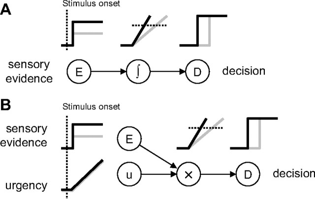
Several widely accepted models of decision making suggest that, during simple decision tasks, neural activity builds up until a threshold is reached and a decision is made. These models explain error rates and reaction time distributions in a variety of tasks and are supported by neurophysiological studies showing that neural activity in several cortical and subcortical regions gradually builds up at a rate related to task difficulty and reaches a relatively constant level of discharge at a time that predicts movement initiation. The mechanism responsible for this buildup is believed to be related to the temporal integration of sequential samples of sensory information. However, an alternative mechanism that may explain the neural and behavioral data is one in which the buildup of activity is instead attributable to a growing signal related to the urgency to respond, which multiplicatively modulates updated estimates of sensory evidence. These models are difficult to distinguish when, as in previous studies, subjects are presented with constant sensory evidence throughout each trial. To distinguish the models, we presented human subjects with a task in which evidence changed over the course of each trial. Our results are more consistent with "urgency gating" than with temporal integration of sensory samples and suggest a simple mechanism for implementing trade-offs between the speed and accuracy of decisions.

Figure 1.

Two alternative models of simple decisions. A, The bounded integrator model, in which sensory information (E) is integrated over time (∫) and compared with a threshold, resulting in a decision (D). When evidence is strong (black lines), the buildup of activity in the neural integrator is faster and produces a decision earlier in time than when evidence is weaker (gray lines). B, The urgency-gating model, in which sensory information is multiplied by a growing signal related to the urgency to respond (u). The product of these two signals causes buildup of activity that, as in A, is faster for strong evidence (black) than for weak evidence (gray).

Figure 2.

Experimental design. A, Behavioral task. Top row, The subject begins each trial by placing the cursor (plus sign) within the central circle. Second row, Next, the tokens begin to move from the center to one of the two targets at a slow speed (predecision interval: 200 ms between token movements). Third row, The subject makes a choice by moving the cursor. Bottom row, The remaining tokens move more quickly to the targets (postdecision interval: 20 ms in fast blocks and 170 ms in slow blocks) and feedback is given to the subject. B, The temporal profile (thick black line) of the probability of a given target is computed using Equation 5. The time of the decision (vertical dashed line) is computed by subtracting the subject's mean reaction time from movement onset time, allowing computation of the success probability at that moment (horizontal dashed line). C, Profiles of success probability for easy trials (black line) and ambiguous trials (gray line). D, Profiles of success probability for bias-for (black) and bias-against trials (gray).

Figure 3.

Comparison of behavior during fast versus slow blocks, using both correct and error trials. A, Distributions of the decision times of a representative subject. Dark line, Fast block (N = 319). Gray shaded region, Slow block (N = 275). The mean decision time in the fast block (dotted black line; 1105 ± 482 ms) was shorter than in the slow block (dotted gray line; 1664 ± 672 ms) (KS test, p < 10⁻²⁵). B, Cumulative distribution of success probability at the time of the decision during fast (black) and slow (gray) blocks, for the same subject. The mean in the fast block (0.69 ± 0.15) was lower than in the slow block (0.77 ± 0.18) (KS test, p < 10⁻⁹). C, Average decision times of each subject during slow (x-axis) and fast (y-axis) blocks. The pluses indicate the mean and SE for subjects for whom the difference was significant (KS test, p < 0.05). The circles represent subjects for whom the difference was not significant. The arrow indicates the subject shown above. D, Average success probability at decision time of each subject during slow (x-axis) and fast (y-axis) blocks. The format is the same as in C.

Figure 4.

Comparison of behavior during correct easy versus ambiguous trials (Fig. 2 C), embedded in the slow blocks. A, Distribution of decision times for one subject. Dark line, Easy (N = 42). Gray shaded region, Ambiguous (N = 16). The mean decision time in easy trials (1520 ± 421 ms) was shorter than in the ambiguous trials (2223 ± 269 ms) (KS test, p < 10⁻⁸). B, Cumulative distribution of success probability at decision time, which was higher in the easy trials (mean, 0.95 ± 0.03) than in ambiguous trials (mean, 0.60 ± 0.11) (KS test, p < 10⁻¹¹). C, Average decision times for all subjects (same format as Figure 3 C). D, Average success probabilities for all subjects (same format as Figure 3 D).

Figure 5.

Comparison of behavior during correct bias-for versus bias-against trials (Fig. 2 D), embedded in the slow blocks. We exclusively focus on those trials in which decisions were made after the first six token movements. A, Distribution of decision times for one subject. Dark line, Bias-for (N = 42). Gray shaded region, Bias-against (N = 46). The mean decision time in bias-for trials (1885 ± 145 ms) was not significantly different from bias-against trials (1957 ± 191 ms) (KS test, p > 0.05). B, Cumulative distribution of success probability at decision time, which was also not significantly different in bias-for (mean, 0.86 ± 0.06) and bias-against trials (mean, 0.88 ± 0.06) (KS test, p > 0.05). C, Average decision times for all subjects (same format as Figure 3 C). D, Average success probabilities for all subjects (same format as Figure 3 D). E, Profiles of success probability for bias-updown (black) and bias-downup (gray) trials. Note that because these trials were relatively rare, we pooled data across subjects to yield 72 bias-updown and 37 bias-downup trials. F, Distributions of decision times for bias-updown (mean, 1447 ± 233 ms) and bias-downup trials (mean, 1327 ± 223 ms). The difference was not significant.

Figure 6.

A, Comparison of mean decision times (DT) in correct (x-axis) versus error trials (y-axis) across all trials in slow blocks (same format as Figure 3 C). B, Comparison of mean decision times in correct versus error trials using data only from easy trials. Data are shown only for those subjects who made at least one error in easy trials (N = 6). C, Comparison of correct versus error decision times in ambiguous (Ambig.) trials. D, Same for bias-for (BF) trials. E, Same for bias-against (BA) trials. F, For each subject, the lines show the success rate across all trials as a function of the number of tokens that moved before the decision. For clarity, points for which there were fewer than five total trials are omitted. G, Same as F except only for easy trials. H, Same for ambiguous trials. I, Same for bias-for trials (all, regardless of when decision was made). J, Same for bias-against trials.

Figure 7.

Simulations of the six models. For each model, the leftmost three plots compare behavior between easy (E) (blue) and ambiguous (A) (red) trials, and the rightmost three plots compare behavior between bias-for (BF) (blue) and bias-against (BA) (red) trials. The first plot of each triplet shows the simulated neural activity of 10 example trials of each type, as a function of time. The second shows histograms of the decision times as a percentage of all trials in which a choice was made. The third plot shows the success probabilities at decision time as a cumulative percentage. The red and green frames highlight the critical comparisons discussed in the text, with red representing disagreement with data and green representing agreement. The frames in the third column compare success probability in easy versus ambiguous trials (as done in Fig. 4 B), whereas those in the fifth column compare decision times in bias-for and bias-against trials (as done in Fig. 5 A). A, Diffusion model (model 1). The shaded region indicates the time period when there are three tokens in each target during bias-for and bias-against trials. B, Diffusion model with leak (model 2). C, Diffusion model that integrates the change in sensory information (model 3). D, Same as C but with a leak (model 4). E, Urgency-gating model without filtering (model 5). F, Urgency-gating model with a low-pass filter (model 6).

Figure 8.

A, Analysis of SumLogLR at decision time for decisions made at different times, for an individual subject's data from slow blocks (N = 266). For each 200 ms bin, we show the mean (dot), SEM (thick lines), and SD (thin lines) of the SumLogLR at the time the decision was made. The oblique line shows a linear regression through the data (slope, −0.24; intercept, 3.41; R ² = 0.29; p < 10⁻¹⁰), suggesting a decreasing threshold. B, Results of linear regressions for all of the subjects (the subject in A is indicated by the arrow). The solid lines show regressions that were significant (p < 0.05), and the dashed lines show those that were not. C, Slopes of regression lines of individual subjects, comparing regressions from slow blocks (x-axis) versus fast blocks (y-axis). The dots indicate when the regression from the slow block was significant. D, Intercepts of regression lines from slow (x-axis) versus fast (y-axis) blocks.

Figure 9.

Neural data from the experiment of Roitman and Shadlen (2002), reprinted with permission. A, Data from the FD version of the motion discrimination task. The solid lines show average neural activity of 54 LIP cells during trials in which the monkey correctly selected the target in the response field of the cell, and the dotted lines show activity when the monkey correctly selected the opposite target. Different colors indicate trials with different motion coherence (see inset). The data on the left are aligned to the onset of motion, and data on the right to the onset of the saccade. B, Data from the RT version of the task, same format.

References

1. Bogacz R, Gurney K. The basal ganglia and cortex implement optimal decision making between alternative actions. Neural Comput. 2007;19:442–477. - PubMed
1. Bogacz R, Brown E, Moehlis J, Holmes P, Cohen JD. The physics of optimal decision making: a formal analysis of models of performance in two-alternative forced-choice tasks. Psychol Rev. 2006;113:700–765. - PubMed
1. Britten KH, Shadlen MN, Newsome WT, Movshon JA. The analysis of visual motion: a comparison of neuronal and psychophysical performance. J Neurosci. 1992;12:4745–4765. - PMC - PubMed
1. Carpenter RH, Williams ML. Neural computation of log likelihood in control of saccadic eye movements. Nature. 1995;377:59–62. - PubMed
1. Chittka L, Skorupski P, Raine NE. Speed-accuracy tradeoffs in animal decision making. Trends Ecol Evol. 2009;24:400–407. - PubMed
Publication types
LinkOut - more resources