Probabilistic combination of slant information: weighted averaging and robustness as optimal percepts

Abstract

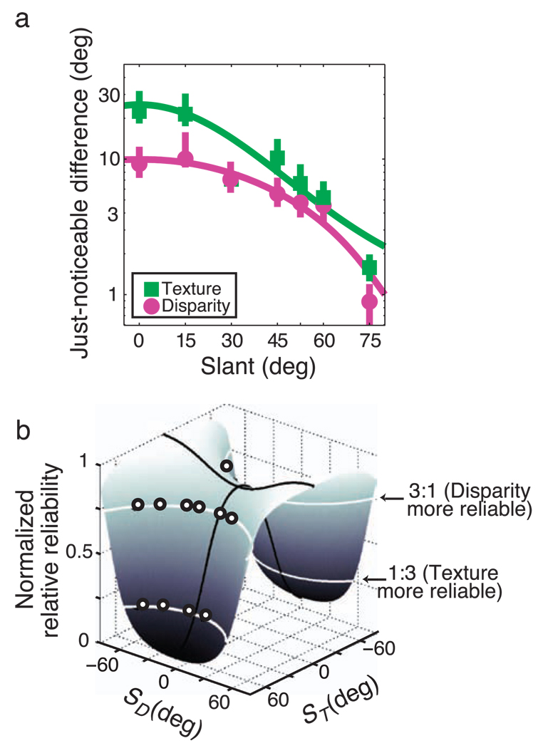
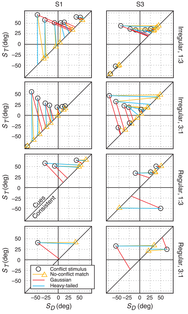
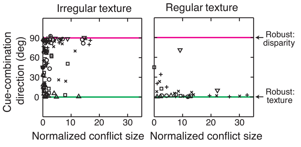
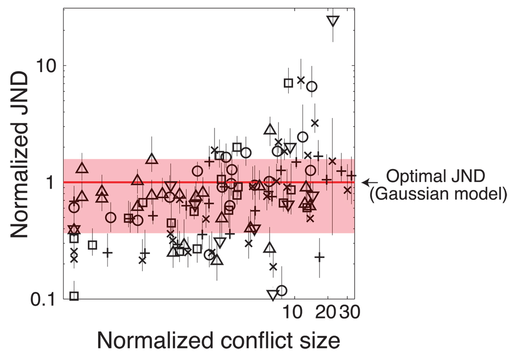
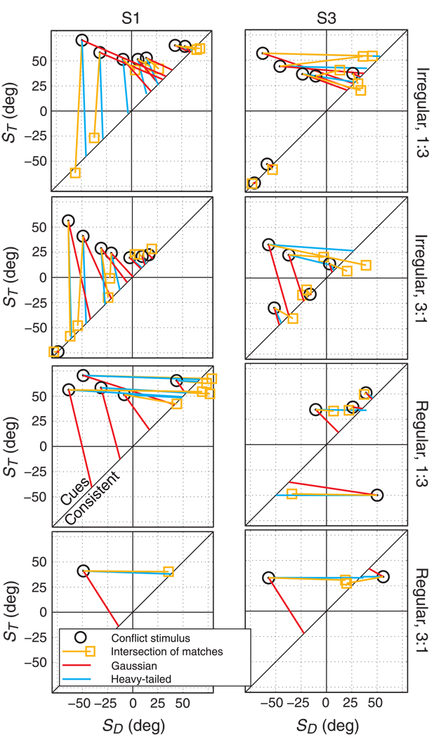
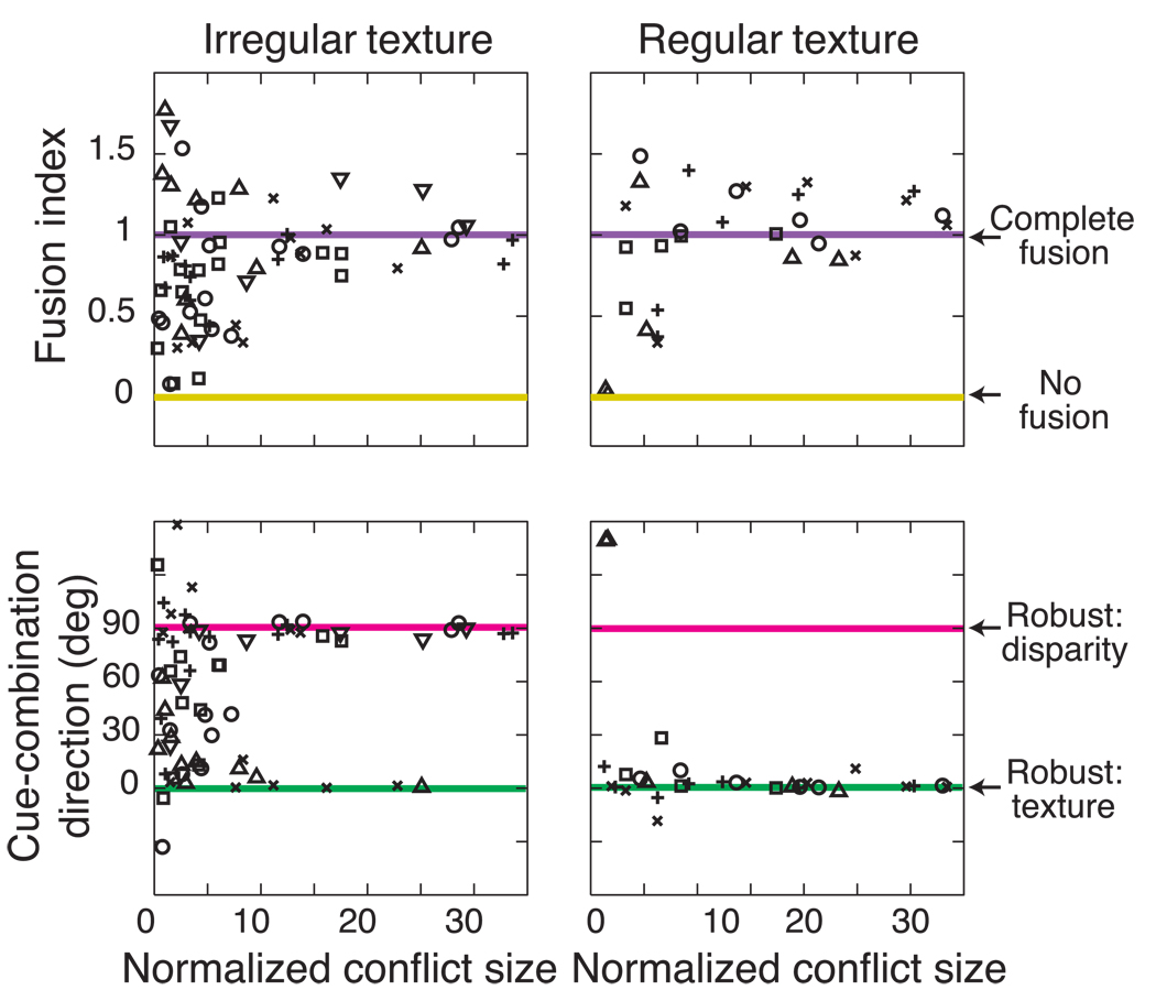
Depth perception involves combining multiple, possibly conflicting, sensory measurements to estimate the 3D structure of the viewed scene. Previous work has shown that the perceptual system combines measurements using a statistically optimal weighted average. However, the system should only combine measurements when they come from the same source. We asked whether the brain avoids combining measurements when they differ from one another: that is, whether the system is robust to outliers. To do this, we investigated how two slant cues-binocular disparity and texture gradients-influence perceived slant as a function of the size of the conflict between the cues. When the conflict was small, we observed weighted averaging. When the conflict was large, we observed robust behavior: perceived slant was dictated solely by one cue, the other being rejected. Interestingly, the rejected cue was either disparity or texture, and was not necessarily the more variable cue. We modeled the data in a probabilistic framework, and showed that weighted averaging and robustness are predicted if the underlying likelihoods have heavier tails than Gaussians. We also asked whether observers had conscious access to the single-cue estimates when they exhibited robustness and found they did not, i.e. they completely fused despite the robust percepts.

Figure 1

a) Gaussian (red) and heavy-tailed (blue) likelihood functions. b–c) The joint likelihoods with disparity-specified slant, S_D, on the horizontal axis and texture-specified slant, S_T, on the vertical axis, assumed to be conditionally independent. Points on the cues-consistent (diagonal) line represent stimuli with the same disparity- and texture-specified slants, whereas points off this line represent stimuli with conflicting slants. Cue-conflict size increases as points get farther from the cues-consistent line. Profiles of the likelihood functions are shown for disparity (above, pink, smaller variance) and texture (left, green, larger variance). Their joint likelihood functions are depicted by gray clouds for which probability (calculated using Equation 1) is proportional to intensity; white dots mark the peaks. The blue dots are the cues-consistent predictions, calculated as the peaks of the intersection profiles of the joint likelihood functions and the cues-consistent axis. b) Gaussian likelihood functions create a joint likelihood function whose profile is elliptical. The cues-consistent prediction is the weighted average as determined by the relative reliabilities of the two cues. c) Heavy-tailed likelihood functions create a joint likelihood function whose profile forms a cross. The cues-consistent prediction is robust and chooses texture because, even though the texture likelihood is more variable, it has less heavy tails.

Figure 2

Experimental stimuli. a) Disparity-only stimulus. Cross-fuse the left and center panels to see the random-dot stimulus in 3D. Or divergently fuse the center and right panels. b) Irregular texture stimulus (monocular). c) Regular texture stimulus (monocular). d) Plan view of the conflict stimuli. The pink line represents the disparity-specified slant and the green line the texture-specified slant. They differ by 2ΔS.

Figure 3

Just-noticeable differences and relative reliabilities. a) JNDs as a function of slant for representative observer S1. Pink circles and green squares represent disparity and texture, respectively. We fit curves to the disparity JNDs by first converting the data to horizontal-size ratios (HSR), defined as α_L/α_R where α_L and α_R are the horizontal angles subtended by a surface patch in the left and right eyes, respectively. The data were then fitted with a line in log space with two free parameters such that JND = ω exp(βHSR) (Hillis et al., 2004). The texture JNDs were fit with a scaled Gaussian with two free parameters: JND = θN(0, ϕ). b) Relative reliability surface for same observer. Normalized relative reliability is plotted as a function of the disparity- and texture-specified slants, where normalized reliability is r_D/(r_D + r_T) for r_i = 1/σ_i². The normalized reliability is a re-writing of the reliability ratio, r_D:r_T that allows us to plot it between 0 and 1. Using the JNDs from a, we computed r_D and r_T (see text). For each possible combination of disparity and texture slants, we computed the normalized relative reliability for the various combinations of disparity- and texture-specified slants. The surface shows the cue conflicts for which disparity is most reliable (peaks) and for which texture is most reliable (troughs). Intersections of the surface and planes parallel to the floor create contours of constant relative reliability. The white lines show two such contours of interest: the desired relative reliability ratios of 3:1 (top line, disparity more reliable) and 1:3 (bottom line, texture more reliable). Points along these contours have constant reliability ratios, but varying conflict sizes. The white circles indicate the conflict conditions used in the experiment. This procedure was done separately for each observer.

Figure 4

Predictions and results of Experiment 1 for observer S1 (left column) and S3 (right column). Each row represents a different condition. Rows 1 and 3 represent conditions in which the relative reliability ratio was 1:3 (texture more reliable) and rows 2 and 4 represent conditions in which the ratio was 3:1 (disparity more reliable). The first two rows represent data when the texture was irregular and the last two represent data when the texture was regular. Note that we were able to achieve the same reliability ratios with irregular and regular textures with the same slants by adjusting the distance to the disparity stimulus. Each panel plots disparity-specified and texture-specified slant on the horizontal and vertical axes, respectively. Black circles represent the conflict stimuli and yellow triangles the no-conflict stimuli that had the same perceived slant as the conflict stimuli; the yellow lines connect the appropriate stimulus pairs. The red lines connect the conflict stimuli with the no-conflict stimuli that the Gaussian likelihood model predicts to have the same perceived slant. The blue lines connect the conflict stimuli with the no-conflict stimuli that the heavy-tailed model predicts to have the same perceived slant.

Figure 5

Cue-combination directions in Experiment 1 for all observers. The left and right panels are for the irregular and regular textures, respectively. Different symbols represent the data from the six observers (S1: ○, S2: x, S3: △, S4: □, S5: +, S6: ▽). The horizontal axis is normalized conflict size (conflict size divided by the pooled standard deviation, $\sqrt{{\sigma }_D^2+{\sigma }_T^2}$, for the two cues, akin to d-prime). The cue-combination direction is the angle between the data vector in Figure 4 and the horizontal axis. The robust choosing disparity prediction is at 0° (pink horizontal line). The robust choosing texture prediction is at 90° (green horizontal line). The predictions for the Gaussian model would be horizontal lines at 60° for cases in which disparity was more reliable (3:1) and 30° for cases in which texture was more reliable (1:3).

Figure 6

Analysis of the results from Experiment 1. Goodness of fit is plotted for each observer and model. The left panel shows the outcome with irregular textures, and the right panel the outcome with regular textures. Goodness of fit was calculated by measuring the sum of squared error between the data and predictions for each of the seven models. Those errors were then normalized, separately for each observer, with the psychometric-fitting and coin-flipping models providing the upper and lower bounds, respectively. The number of free parameters for each model is indicated in parentheses.

Figure 7

JND data from Experiment 1 for all observers. Normalized JND is plotted as a function of normalized conflict size. We normalized each JND by dividing by the optimal JND for that conflict stimulus. The optimal JND was calculated using the corresponding single-cue JNDs determined from the relative reliability surface and the Gaussian-likelihood model: $\sqrt{{\sigma }_{D1}^2{\sigma }_{T1}^2/({\sigma }_{D1}^2+{\sigma }_{T1}^2)}$. Error bars are 95% confidence intervals. The abscissa is on a log scale; normalized conflicts of 0 are plotted at 0.1. Different symbols represent the data from the six observers (S1: ○, S2: x, S3: △, S4: □, S5: +, S6: ▽). The red horizontal line indicates a normalized JND of 1, the point of optimal performance with the Gaussian-likelihood model; the mean region of 95% confidence is shown in light red.

Figure 8

Predictions and results of Experiment 2 for observer S1 (left column) and S3 (right column). Rows 1 and 3 represent conditions in which the relative reliability ratio was 1:3 (texture more reliable) and rows 2 and 4 represent conditions in which the ratio was 3:1 (disparity more reliable). The first two rows represent data when the texture was irregular and the last two represent data when the texture was regular. Each panel plots disparity-specified and texture-specified slant on the horizontal and vertical axes, respectively. Black circles represent the two-cue, conflict stimuli. The single-cue stimuli that perceptually matched the two-cue stimuli can be visualized as horizontal (texture-only) and vertical (disparity-only) lines (not shown). Yellow squares represent the intersection of these two lines, and thus represent two settings at once. Yellow lines connect those matching stimuli. The red lines represent the predictions of the Gaussian model (see Discussion); the positions where those lines intersect the cues-consistent line represent the predicted matches if complete fusion occurred; matches consistent with partial fusion lie along the same lines, but closer to the two-cue conflict stimulus. The blue lines represent the predictions of the heavy-tailed model (see Discussion); matches consistent with complete fusion lie at the intersection of those lines and the cues-consistent line; matches consistent with partial fusion are on the same lines, but closer to the two-cue conflict stimulus.

Figure 9

Summary of results in Experiment 2 for all observers. The upper row shows the observed amount of fusion relative to the no-fusion and complete-fusion predictions. The fusion index (see text) is plotted as a function of normalized conflict size. An index of 0 indicates no fusion (yellow horizontal line). An index of 1 indicates complete fusion (yellow purple line). The left and right columns are for the irregular and regular textures, respectively. Different symbols represent the data from the six observers (S1: ○, S2: x, S3: △, S4: □, S5: +, S6: ▽). The second row shows cue-combination directions as a function of normalized conflict size. The robust choose-disparity prediction is 0° (pink horizontal line), indicating the match was determined entirely by the texture signal. The robust choose-texture prediction is 90° (green horizontal line), indicating the match was determined entirely by the disparity signal. The Gaussian predictions would be horizontal lines at 60° when disparity was more reliable (3:1, according to the Gaussian model) and at 30° when texture was more reliable (1:3).

Figure 10

Relative goodness of fit for various models of Experiment 2. The abscissa represents the six observers. The ordinate represents the goodness of fit, computed as in Figure 6. Dark red, medium red, red, dark blue, blue, and light blue represent the goodness of fit respectively for the various models: Gaussian no-fusion, Gaussian partial-fusion, Gaussian complete-fusion, heavy-tailed no-fusion, heavy-tailed partial-fusion, and heavy-tailed complete-fusion. The number of free parameters is indicated in parentheses. The left panel shows the data when the texture was irregular and the right panel the data when it was regular. The dashed lines represent the fits for the psychometric and coin-flipping models, which respectively represent upper and lower bounds for goodness of fit.

Figure 11

JND data from Experiment 2 for all observers. Normalized JND is plotted as a function of normalized conflict size, as in Figure 7. Gray symbols represent the data from disparity-only matches and black symbols data from texture-only matches.

References

1. Alais D, Burr D. The ventriloquist effect results from near-optimal bimodal integration. Current Biology. 2004;14:257–262. - PubMed
1. Arnold RD, Binford TO. Geometric constraints in stereo vision. SPIE: Image Processing for Missile Guidance. 1980;238:281–292.
1. Backus BT, Banks MS, van Ee R, Crowell JA. Horizontal and vertical disparity, eye position, and stereoscopic slant perception. Vision Research. 1999;39:1143–1170. - PubMed
1. Banks MS, Backus BT. Extra-retinal and perspective cues cause the small range of the induced effect. Vision Research. 1998;38:187–194. - PubMed
1. Box GEP, Tiao GC. Bayesian inference in statistical analysis. New York: John Wiley & Sons; 1992. Wiley Classics Library edition.
Publication types