Transformation of polarized light information in the central complex of the locust

Abstract

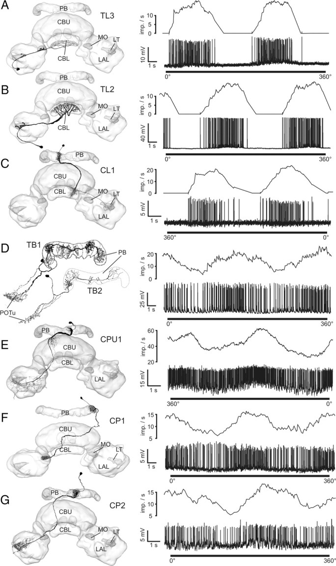
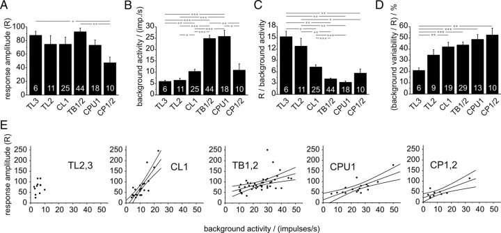
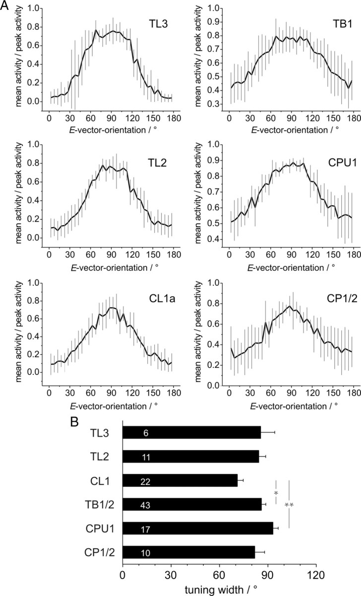
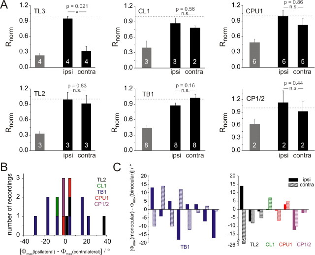
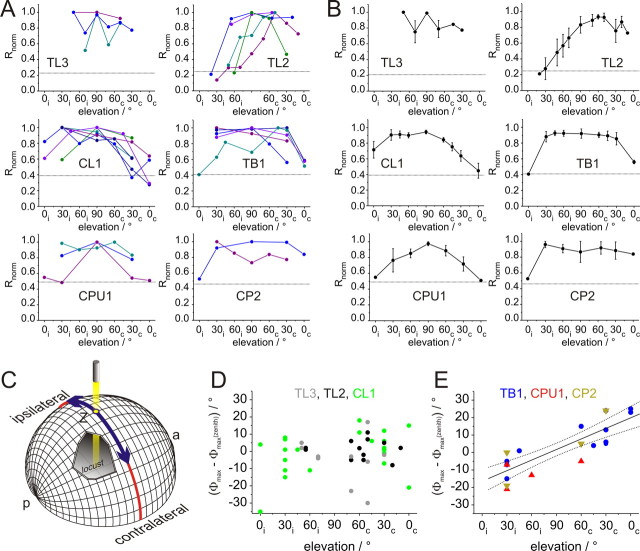
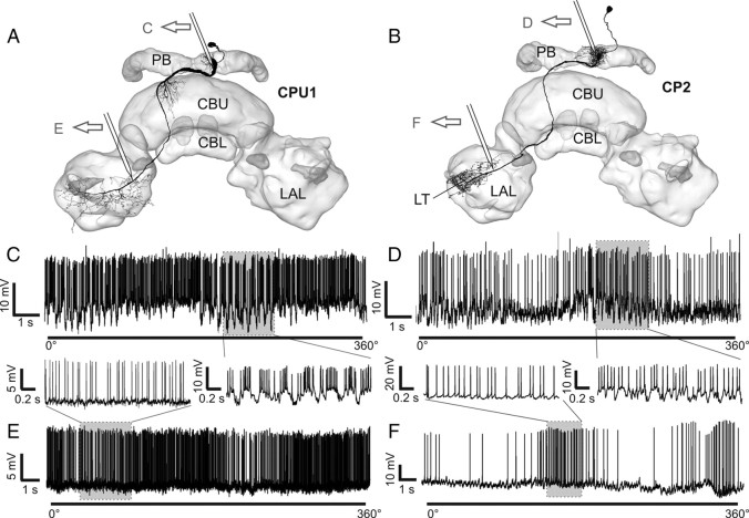
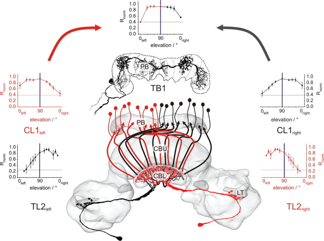
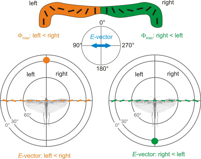
Many insects perceive the E-vector orientation of polarized skylight and use it for compass navigation. In locusts, polarized light is detected by photoreceptors of the dorsal rim area of the eye. Polarized light signals from both eyes are integrated in the central complex (CC), a group of neuropils in the center of the brain. Thirteen types of CC neuron are sensitive to dorsally presented, polarized light (POL-neurons). These neurons interconnect the subdivisions of the CC, particularly the protocerebral bridge (PB), the upper and lower divisions of the central body (CBU, CBL), and the adjacent lateral accessory lobes (LALs). All POL-neurons show polarization-opponency, i.e., receive excitatory and inhibitory input at orthogonal E-vector orientations. To provide physiological evidence for the direction of information flow through the polarization vision network in the CC, we analyzed the functional properties of the different cell types through intracellular recordings. Tangential neurons of the CBL showed highest signal-to-noise ratio, received either ipsilateral polarized-light input only or, together with CL1 columnar neurons, had eccentric receptive fields. Bilateral polarized-light inputs with zenith-centered receptive fields were found in tangential neurons of the PB and in columnar neurons projecting to the LALs. Together with other physiological parameters, these data suggest a flow of information from the CBL (input) to the PB and from here to the LALs (output). This scheme is supported by anatomical data and suggests transformation of purely sensory E-vector coding at the CC input stage to position-invariant coding of 360 degrees -compass directions at the output stage.

Figure 1.

Morphologies of major types of POL-neuron of the locust central complex and their neuronal responses to a 360° rotation of a dorsally presented polarizer. Frontal camera lucida reconstructions, projected onto three-dimensional reconstructions of the central complex, are shown on the left. Spike trains (lower lanes) and mean activities (upper lanes; gliding average, bin size: 1 s) are shown on the right. Morphological and physiological data belong to neurons from the same cell type. A, TL3 neuron. B, TL2 neuron. C, CL1a neuron. D, TB1/2 neurons, physiology from a TB1 neuron. E, CPU1 neuron. F, CP1 neuron. G, CP2 neuron. LT, Lateral triangle; MO, median olive; POTu, posterior optic tubercle. Neuron morphologies are modified from Träger et al. (2008) (A, B), Heinze and Homberg (2008) (C, E–G), Heinze and Homberg (2007) (D, top), and Heinze and Homberg (2009) (D, bottom).

Figure 2.

Response amplitudes and background activities in the different types of POL-neuron. A, Mean response amplitudes of all major types of neuron. B, Background firing rates for each group of neuron. C, Ratios of response amplitude and background firing rate for each group of neuron. This ratio provides an estimate of the information content of the frequency modulations during a rotation of the polarizer. D, Variability in background spiking activity. Means of R values of background activity, normalized to the absolute response amplitude of each neuron, are plotted. The resulting values indicate how much variability during stimulation is due to spontaneous variability. Asterisks indicate significant differences as revealed by ANOVA analysis with Games-Howell post hoc test. Significance levels: *p < 0.05; **p < 0.01; ***p < 0.001. Numbers of recordings are indicated in each bar. Error bars represent SE. E, Relation between response amplitude and background activity. The graphs show all recordings grouped according to main cell type. Linear regression lines (with 95% confidence intervals) are presented for each group of neurons. There was no statistical difference between the linear regressions for TB, CPU1, and CP neurons (test for equality of slopes, using analysis of covariance; p = 0.767). TL neurons did not show significant linear correlation, while the regression line for CL1 neurons was distinct from all remaining regressions (p < 0.001 for all three cell types). Data for linear regressions: TL2/3, p = 0.47, R_cor = 0.23; CL1, p < 0.0001, R_cor = 0.82; TB1,2, p = 0.0014, R_cor = 0.48; CPU1, p = 0.00036, R_cor = 0.76; CP1/2, p = 0.004, R_cor = 0.82.

Figure 3.

Characteristics of tuning curves of different types of POL-neuron. A, Average shapes of tuning curves (means ± SD, bin size: 5°) from five neurons with the largest response amplitude in each category (supplemental Fig. 3, available at www.jneurosci.org as supplemental material). Tuning curves were normalized to peak activity during each rotation, manually aligned, averaged within each recording, and thereafter averaged across neurons. Plots are scaled from minimal to maximal activity. B, Comparison of mean tuning widths at half maximal activation. Numbers of recordings are indicated in each bar. The tuning widths of some recorded neurons could not be determined reliably, because of low response amplitudes and ambiguous values of half maximal activation. Therefore the numbers are lower than in Figures 2A–D. Asterisks indicate significant differences revealed by ANOVA analysis combined with Tukey-HSD post hoc test. Significance levels: *p < 0.05; **p < 0.01. Error bars represent SE.

Figure 4.

Ocular dominance of the different types of POL-neuron. A, Response amplitudes for monocular stimulation with a dorsally rotating polarizer (ipsi, ipsilateral eye only; contra, contralateral eye only). Gray bars indicate mean background variability of the tested neurons. Response amplitudes (R) of each neuron were normalized to the binocular response amplitude (dashed line) before averaging. Numbers of recordings are indicated in each bar. Error bars represent SE. B, Distribution of differences in Φ_max values between stimulations through the ipsi- and contralateral eye. The numbers of recordings are plotted per 3° bins. Negative values indicate that the contralateral Φ_max value is larger than the ipsilateral one. Values are generally distributed symmetrically around zero.TB1 neurons exhibit larger differences than the remaining cell types. C, Deviations of monocular Φ_max values from binocular values. Each pair of bars (hatched and filled) represents ipsilateral (filled) and contralateral (hatched) values from one neuron. TB1 neurons are presented in the left graph, all remaining cell types in the right graph. In most TB1 neurons binocular values were between the monocular stimulations, whereas this occurred only once in all remaining cell types.

Figure 5.

Receptive field properties of POL-neurons. A, Response amplitudes of the different types of POL-neuron plotted against elevation of polarized-light stimulus. Elevation is plotted with respect to the location of the soma and was sampled along the meridian orthogonal to the longitudinal body axis of the locust. Values were normalized to the largest R value of each neuron (i.e., the receptive field center). Individual recordings are distinguished by different colors. Data points are connected by lines for better visibility. Dotted lines indicate background variability for each neuron type (from Fig. 4), which have been renormalized with respect to the mean receptive field center in each cell type. B, Average receptive fields for the examined groups of POL-neurons. Dotted lines, background variability. Values are means ± SE. Missing values in individual recordings were interpolated linearly to allow for averaging at all elevations. C, Schematic representation of stimulus display. The locust is located in the center of the sphere, oriented along the anterior (a)–posterior (p) axis. Stimuli were moved along the meridian (blue) orthogonal to the body axis. Ipsi- and contralateral refer to neurons with cell body in the left hemisphere of the brain. D, E, Deviations of Φ_max values at different elevations from zenithal Φ_max values for TL3, TL2, and CL1 neurons (D), and for TB1, CPU1, and CP2 neurons (E). Differences in Φ_max values are plotted against elevation. A significant correlation was observed for the combined values of TB1, CPU1, and CP1 (R_cor = 0.84, t test against the slope of 0, p < 0.00001), indicated in E by the regression line with 95% confidence intervals. No correlation was observed for neurons in D (R_cor = 0.19, p = 0.23).

Figure 6.

Indication of presynaptic and postsynaptic arborizations by recordings from different regions of CPU1 and CP2 neurons. A, B, Frontal reconstructions of a CPU1 (A) and CP2 neuron (B), projected onto a three-dimensional reconstruction of the CC. Approximate recording sites of the recording traces in C–F are indicated. C, Recording trace from arborizations of a CPU1 neuron in the PB during zenithal rotation of the polarizer. Postsynaptic, graded potentials are visible (enlargement of shaded area is shown in the inset). D, Recording trace from PB-arborizations of a CP2 neuron during a rotation of the polarizer. Postsynaptic potentials are clearly visible (enlarged in the inset). E, F, Recording traces obtained from the vicinity of the LAL from a CPU1 neuron (E) and a CP2 neuron (F). Enlargements emphasize the even baseline without major graded potential changes. LT, Lateral triangle. Neuron morphologies in A and B are modified from Heinze and Homberg (2008).

Figure 7.

Model of neuronal wiring principles derived from receptive field data superimposed on a three-dimensional reconstruction of the central complex. Input neurons (TL2) have relatively small, contralaterally centered receptive fields, i.e., neurons in the left brain hemisphere have receptive fields centered in the right sky hemisphere (black) and vice versa for the right brain hemisphere (red). CL1 neurons have slightly larger, ipsilaterally centered receptive fields, implying midline crossing connections between TL2 and CL1 neurons (colors indicate the source of polarized light information). CL1 neurons are represented by arrows following the anatomical trajectories of CL1 cells. The smooth arborizations of TB1 neurons (top, projections to the posterior optic tubercle omitted) on either side of the PB-midline provide the potential targets for CL1 cells. Therefore, the bilaterally symmetrical receptive fields of TB1 neurons can be explained by integration of signals from at least two CL1 cells, one from each hemisphere. The morphology of the TB1 neuron is modified from Heinze and Homberg (2007).

Figure 8.

Schematic illustration of a potential mechanism for resolving the azimuthal ambiguity through E-vector signaling in columnar neurons of the PB, based on Φ_max distributions in the receptive fields. The top panel shows the polarotopic representation of zenithal E-vectors in the columns of the PB. As neurons comprising this representation show smaller Φ_max values for stimuli presented in the ipsilateral sky hemisphere, neurons of the left brain side prefer stimulus situations with E-vectors in the left half of the sky to be smaller than in the right half. Accordingly, neurons of the right brain hemisphere prefer stimulus situations, in which E-vectors in the right half of the sky are smaller than in the left half. These two stimulus situations occur in the sky, when the sun is either behind the locust (bottom right), or in front of the locust (bottom left). Therefore, neurons in the left PB-hemisphere would be more strongly activated, when the sun is in front of the animal, whereas neurons in the right PB-hemisphere react more strongly when the sun is behind the locust. Note that the zenithal E-vectors are identical in both situations. E-vector angles in the sky at different elevations are derived from Petzold (2001).

References

1. Clements AN, May TE. Studies on locust neuromuscular physiology in relation to glutamic acid. J Exp Biol. 1974;60:673–705. - PubMed
1. Heinze S, Homberg U. Maplike representation of celestial E-vector orientations in the brain of an insect. Science. 2007;315:995–997. - PubMed
1. Heinze S, Homberg U. Neuroarchitecture of the central complex of the desert locust: Intrinsic and columnar neurons. J Comp Neurol. 2008;511:454–478. - PubMed
1. Heinze S, Homberg U. Linking the input to the output: new sets of neurons complement the polarization vision network of the locust central complex. J Neurosci. 2009;29:4911–4921. - PMC - PubMed
1. Homberg U. Neuroarchitecture of the central complex in the brain of the locust Schistocerca gregaria and S. americana as revealed by serotonin immunocytochemistry. J Comp Neurol. 1991;303:245–254. - PubMed
Publication types
LinkOut - more resources