

Review
doi: 10.1021/cr900095e.
Normal mode analysis of biomolecular structures: functional mechanisms of membrane proteins
Affiliations
- PMID: 19785456
- PMCID: PMC2836427
- DOI: 10.1021/cr900095e
Item in Clipboard
Review
Normal mode analysis of biomolecular structures: functional mechanisms of membrane proteins
Chem Rev.
.
No abstract available
Figures
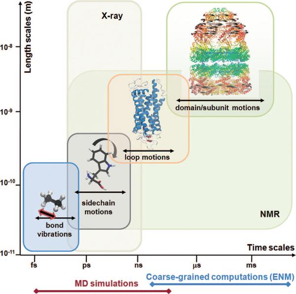
Equilibrium motions of proteins. Motions accessible near native state conditions range from femtoseconds (bond length vibrations) to milliseconds or slower (concerted movements of multiple subunits; passages between equilibrium substates). X-ray crystallographic structures span length scales up to several hundreds of angstroms. Fluctuations in the subnanosecond regime are indicated by X-ray crystallographic B-factors. NMR spectroscopy is restricted to relatively smaller structures, but NMR relaxation experiments can probe a broad range of motions, from picoseconds to seconds, including the microseconds time range of interest for several allosteric changes in conformation. Also indicated along the abscissa are the time scales of processes that can be explored by MD simulations and coarse-grained computations. Molecular diagrams here and in the following figures have been generated using Jmol (http://www.jmol.org/ ), PyMol (http://www.pymol.org/ ), or VMD visualization software.
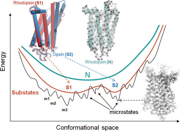
Energy profile of the native state modeled at different resolutions. N denotes the native state, modeled at a coarse-grained scale as a single energy minimum. A more detailed examination of the structure and energetics reveals two or more substates (S1, S2, etc.), which in turn contain multiple microstates (m1, m2, etc.). Structural models corresponding to different hierarchical levels of resolution are shown: an elastic network model representation where the global energy minimum on a coarse-grained scale (N) is approximated by a harmonic potential along each mode direction; two substates S1 and S2 sampled by global motions near native state conditions; and an ensemble of conformers sampled by small fluctuations in the neighborhood of each substate. The diagrams have been constructed using the following rhodopsin structures deposited in the Protein Data Bank: 1U19 (N); 1U19 and 3CAP (S1 and S2); and 1F88, 1GZM, 1HZX, 1L9H, 1U19, 2G87, 2HPY, 2I35, 2I36, 2I37, 2J4Y, 2PED, 3C9L, and 3C9M (microstates).
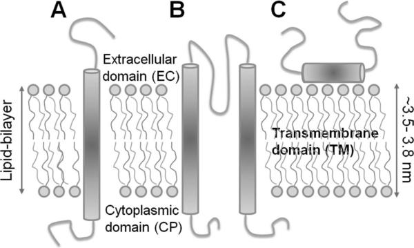
Schematic representation of different types of integral membrane proteins. (A) Single helical TM protein (a bitopic membrane protein), (B) a polytopic TM protein composed of multiple TM elements (here two helices), and (C) an integral monotopic membrane protein.
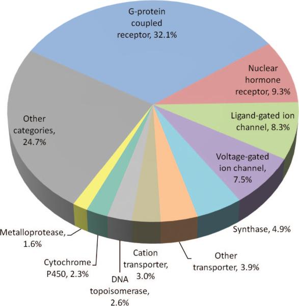
Distribution of small molecule drugs based on the targeted molecular function. The distribution is shown for the top-ranking ten functional categories targeted by 965 FDA-approved small molecule drugs, excluding biotechnology drugs, nutraceuticals such as vitamins and amino acids, and those with uncertain targets. The top ten categories shown in the pie chart are associated with more than 75% of the drugs in the data set. The distribution is based on 1008 drug–protein associations. A given category is counted once if a given drug targets multiple proteins in that category.
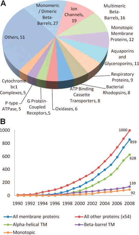
PDB statistics for membrane proteins. (A) Structures of 182 unique membrane proteins are available in the PDB, as of January 2009. The pie chart displays the distribution of these structures among different functional/structural categories. (B) Growth of released membrane protein structures and other protein structures starting from 1990. Note that the number of “other” proteins is reduced by a factor of 54 in the curve, for display purposes. We also show the breakdown of membrane proteins into different structural groups: α-helical TM, β-barrel TM, and monotopic. An exponential growth with an R2 value of 0.99 is observed in the last ten years for both membrane proteins and all other proteins. The corresponding growth rates are 0.23 and 0.18, respectively; that is, they are higher for membrane proteins due to initiatives in that direction.
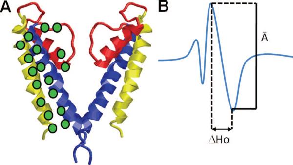
Site-directed spin-labeling coupled with EPR illustrated for a potassium channel. (A) Molecular model of KcsA (omitting two of the four subunits for clarity). The green discs indicate the positions of the spin-labeled residues (probes) on TM1 (yellow), TM2 (blue), and the selectivity filter (red). (B) Measurement of the structural parameter from the spectral line shape of an EPR-spectrum. The amplitude (A–) of the normalized central resonance line M = 0 and the mobility parameter ΔHo (the peak-to-peak width at M = 0) are shown. Changes in two structural parameters are usually examined: (i) probe mobility (ΔHo) and (ii) spin–spin interaction parameter W. Changes in the probe mobility, ΔΔHo, indicate rearrangements in tertiary or quaternary contacts, while the W parameter obtained from the ratio of the normalized amplitude spectra (A–) in different forms reports changes in the intersubunit probe-to-probe proximity. Such measurements performed by Perozo and co-workers for the open and closed conformations of KcsA as a function of pH revealed the coupled rigid-body rotations of TM helices TM1 and TM2 of the four subunits and the opening of the permeation pore (gating) induced by the concerted rotations of the TM2 helices while the selectivity filter remained practically immobile.
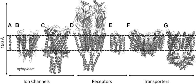
Transmembrane proteins studied by NMA, considered in the present review: (A) gramicidin A, (B) KcsA, (C) MscL, (D) nAChR, (E) rhodopsin, (F) glutamate transporter (Gltph), and (G) BtuCD. The bilayer is indicated by the dashed lines. The ribbon diagrams were constructed using the respective structures 1NRU, 1K4C, 2OAR, 2BG9, 1L9H, 1XFH, and 1L7V available in the PDB.
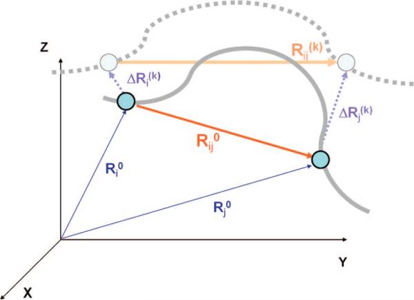
Schematic view of interaction sites and their displacements. In the initial conformation, CG sites i and j are located respectively at Ri0 and Rj0, and the vector Rij0 = Rj0 – Ri0 defines the distance vector between these sites. Upon displacement along mode k, the CG sites move to Ri0 + ΔRi(k) and Rj0 + ΔRj(k), and the distance vector becomes Rij(k). The solid gray line represents the structural details of the initial-state protein that are above the resolution of the coarse graining, and the broken gray line indicates the structure after a displacement along mode k.
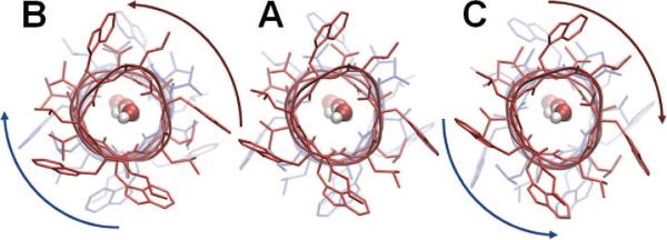
Counter-rotations of the two helical dimers of gramicidin A, viewed from the EC side along the channel axis. This is the lowest frequency ANM mode of motion of the dimer. It is accompanied by a lateral expansion at the helical termini near the CP and EC regions. This mode was found to be crucially important for the initiation of the dissociation of the monomers needed for ion channel gating. Calculations were performed on an ANM server (http://ignmtest.ccbb.pitt.edu/cgi-bin/anm/anm1.cgi ), using the PDB structure 1JNO. Panel A displays the PDB structure, and panels B and C show two conformations fluctuating in opposite directions along the lowest frequency mode. Water molecules were placed inside the pore using Sybyl 8.3. (figure inspired by ref 192).
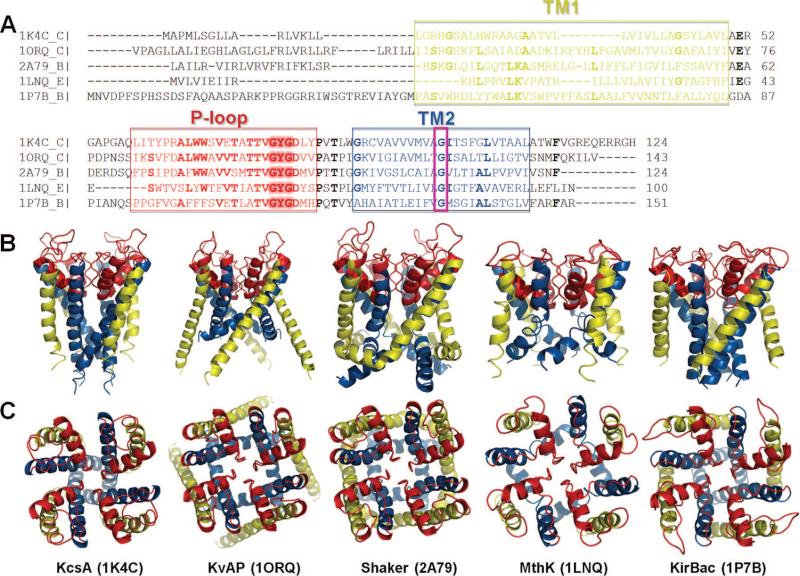
Sequence and structure of the pore region of five structurally known K+ channels. (A) Alignment of the pore region sequences. The regions corresponding to the helices TM1 and TM2 and the P-loop are indicated by the boxed green, blue, and red letters, respectively. The alignment was performed using ClustalW. Fully or highly conserved amino acids are written in boldface. Two regions of interest are the signature motif GYG (highlighted) at the selectivity filter and the conserved glycine on TM2 (e.g., G83 in MthK) enclosed in a magenta box. (B and C) Structural comparison of the pore forming regions aligned in panel A. These are all tetrameric structures. The monomers contain either two TM helices (KcsA, MthK, and KirBac, with PDB ID's 1K4C, 1LNQ, and 1P7B, respectively) colored yellow (TM1) and blue (TM2) or six TM helices (KvAP and Shaker with PDB ID's, 1ORQ and 2A79, respectively). The helices S5 and S6 of KvAP and Shaker are equivalent to the respective helices TM1 and TM2 of the other K+ channels and are displayed here, along with the P-loop region, colored red. The channels are viewed from side (B) and from the top (EC region) (B) (see ref for more details).
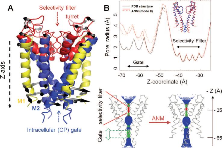
Opening up of the potassium channel pore by the global twisting mode. (A) Ribbon diagram of KcsA illustrating the basic structural regions and the motion along the second slowest ANM mode. This is a global twisting (nondegenerate) mode that induces counter-rotations at the EC and CP regions, indicated by the white/gray arrows. (B) Top panel: The pore-radius profile as a function of the pore axis (Z-axis), calculated for the X-ray structure (black curve) and for two conformations visited by fluctuations in opposite directions along the global twisting mode (red curves). The inset shows the backbone trace of two of the monomers in the X-ray structure (blue) and the ANM-predicted conformation (red). The separation between the inner (TM2) helices at the gate is enlarged by about 1.5 Å. Bottom panel: A mesh-wire representation of the channel pore before (left) and after (right) reconfiguration along the second ANM mode. Color code: blue, radius > 3 Å; green, 3 Å > radius > 2 Å; red, radius < 2 Å. For visual clarity, only two monomers of the tetramer are shown (see ref for more details).
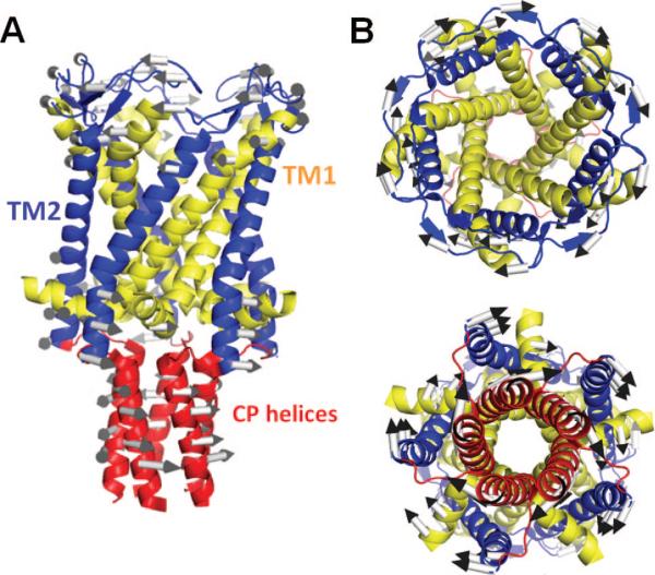
Global dynamics of M. tuberculosis MscL predicted by the ANM. (A) Side view of the pentameric structure, and (B) views from the EC (top) and CP (bottom) regions. The TM helices are colored yellow (TM1) and blue (TM2), which are the inner and outer helices, respectively. CP helices are colored red. The TM and CP helices rotate in opposite directions in the slowest ANM mode. The directions of the arrows in panel B refer to the rotations as viewed from the EC and CP regions, hence their “apparent” rotation in the same direction. We also note that the structure fluctuates between two conformers where the TM helices and CP helices undergo counter-rotations, in either direction; that is, the arrows displayed in the figure represent one of the two opposite direction movements along this mode axis. The ribbon diagrams are generated using the structure (PDB ID: 2OAR) resolved by Chang et al.
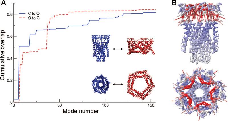
Cumulative contribution of ANM modes to the structural change between the open and closed forms of MscL. The ordinate displays the cumulative overlap between the ANM modes (eigenvectors) predicted for the starting conformation and the targeted direction of structural change. ANM calculations were performed using either the closed (C) form (blue, solid curve) or open (O) form (red, dashed) as the starting substate. In either case, a cumulative overlap of about 0.8 is achieved by the top-ranking ~120 modes (less than 1/10th of accessible modes). Concrete (stepwise) contributions are made by the nondegenerate modes. The 2nd lowest nondegenerate mode accessible to the closed form (mode 6) is illustrated in panel B. This mode induces a contraction/expansion along the pentameric axis, mainly the portion close to the EC region, as seen from the side (top) and EC (bottom) views of the channel.
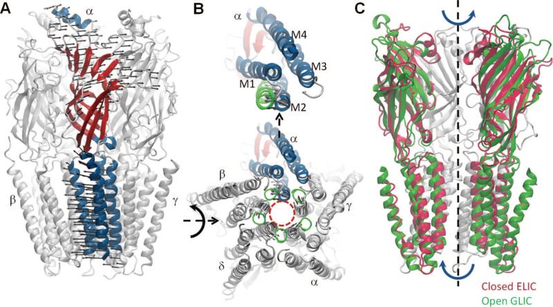
Ligand-gated ion channel nAChR structure and dynamics. (A) Structure of the EC and TM domains of nAChR (PDB ID: 2BG9). The secondary structure of one of the monomers (α) is colored to display the β-sandwich fold (red) of the EC domain and the four TM helices (M1–M4; blue) of the TM domain; and the remaining four monomers are shown in gray. The lowest frequency ANM mode induces a quaternary symmetric twist, as indicated by the arrows shown for monomer α. (B) CP end of TM domain (bottom) and close up view of one of the monomers (monomer α, colored) (top). Red dashed circle indicates the channel pore. Arrows indicate the collective movements of M2 helices along ANM mode 1. Green circles represent the CP end of the M2 helices after deformation along ANM mode 1. (C) Comparison of bacterial homopentameric LGICs ELIC (2VL0) and GLIC (3EAM) shows the contribution of this quaternary twist mode to the conformational changes involved in activation. One subunit (closest to the viewer) is omitted to display the channel pore.
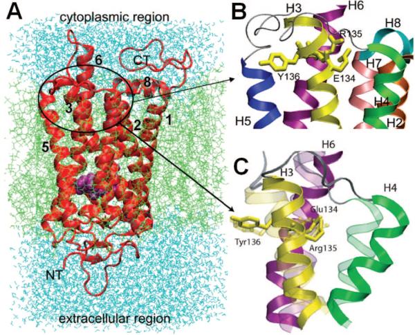
Rhodopsin structure and its ERY motif at the CP region. (A) Ribbon diagram of the first rhodopsin structure determined by Palczewski and co-workers, shown in a lipid bilayer. This is a seven TM helix structure, enclosing a chromophore (cis-retinal, shown in space filling, magenta). The C- and N-termini are labeled as CT and NT, along with some of the TM helices that can be distinguished clearly. Note that there is an eighth helix, at the CP region, that runs parallel to the membrane surface. (B) Enlarged view of the CP region containing the ERY motif (E134–R135–Y137) on the TM helix 3 (or H3), involved in G-protein recognition. (C) Reconfiguration of the ERY-motif-containing domain upon cis–trans isomerization of the retinal induced by light activation, suggested by an ANM analysis of rhodopsin dynamics.
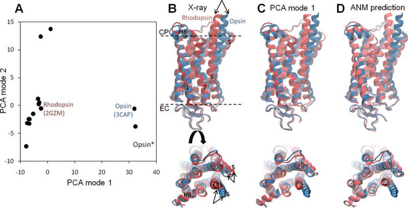
PCA and ANM calculations for rhodopsin. (A) Distribution of 16 X-ray structures in the subspace spanned by the PCA mode directions 1 and 2. These respective modes account for 62% and 12% of the structural variability in the data set. The principal axis 1 differentiates the inactive and (putative) activated structures which are clustered in two distinctive groups, and the PCA axis 2 further differentiates between the structures in the cluster of inactive rhodopsins (B). Superimposition of experimentally determined rhodopsin and opsin structures, indicated by the labels on panel A. (C) Rhodopsin structure generated by deforming the opsin structure along the first principal mode, p1. (D) Rhodopsin conformation predicted by deforming the opsin structure along the 20 lowest frequency ANM modes. The 14 rhodopsin structures in the analyzed set include, in addition to the ground state,– and various photoactivated states, lumirhodopsin, bathorhodopsin, 9-cis-rhodopsin, photoacivated deprotonated intermediate, and thermostabilized mutants., These microstates are dispersed along the second principal axis. These calculations have been performed for the Cα atoms only; the remaining backbone atoms were reconstructed with the BioPolymer module of Sybyl 8.3 (Tripos). ANM calculations were performed using the relatively short cutoff distance of Rc = 8 Å, so as to release interhelical constraints.
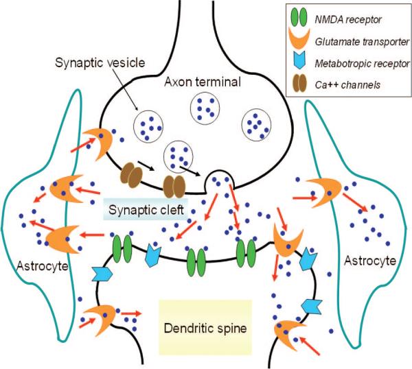
Release, uptake, and reuptake of glutamate at an excitatory synapse. Upon arrival of an action potential at the presynaptic axon terminus, voltage-sensitive Ca2+ channels trigger the fusion of vesicles with the cell membrane to release glutamate molecules in the synaptic cleft. Glutamates bind and activate receptors on the postsynaptic cell membrane. Excess glutamate is cleared by glutamate transporters, which are more abundant and efficacious in the glia in the vicinity of the synapse.
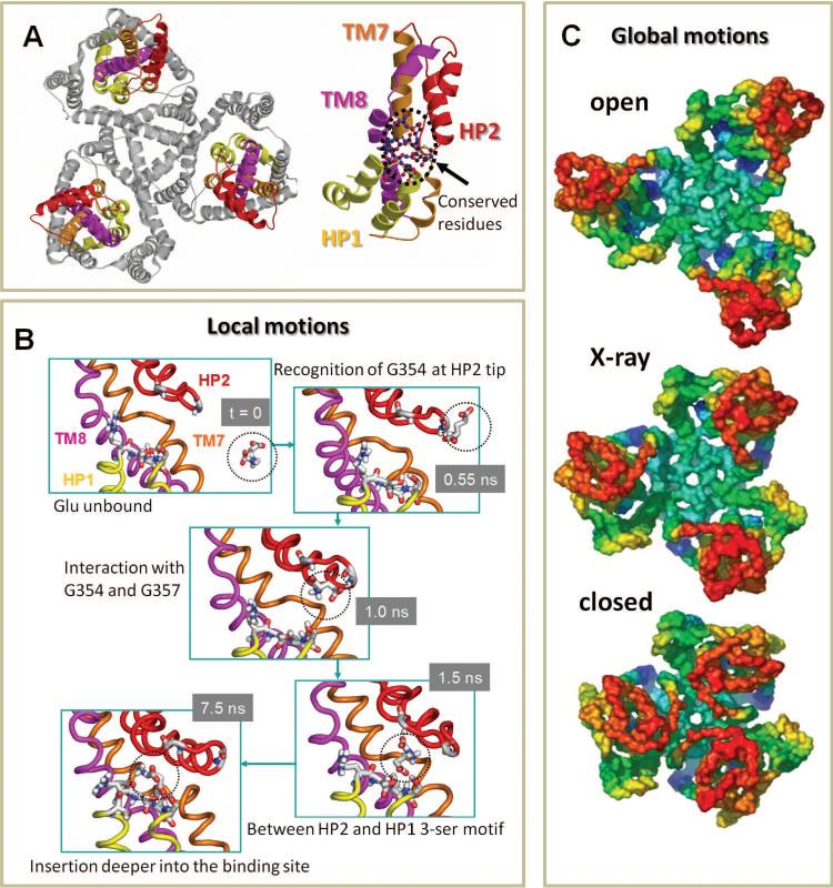
Structure and dynamics of glutamate transporter. (A) The homotrimer, viewed from the EC region. The N-terminal region (TM1–TM6) is displayed in gray; the C-terminal core HP1–TM7–HP2–TM8 is colored yellow–orange–red–violet and labeled in the figure on the right. (B) Snapshots from MD simulations, illustrating the time-resolved recognition and binding events, starting from t = 0, where the substrate is in the aqueous cavity, up to t = 7.5 ns, where the substrate is sequestered at the binding site and remains therein for the remaining duration of the simulation, of ~20 ns. (C) Symmetric opening/closing mode of GltPh, as observed in ANM. The middle diagram displays the GltPh structure viewed from the EC side (PDB: 1xfh); the top and bottom diagrams display the ANM-predicted open and closed conformations, respectively. In the X-ray structure, the basin is exposed to the EC aqueous environment, while in the closed form contacts between neighboring subunits occur (see, for example, the L34 loops colored red).
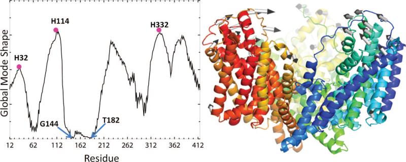
Global dynamics of the aspartate transporter GltPh predicted by the ANM. (A) Distribution of square displacements of residues, (ΔRi)2|1 + (ΔRi)2|2 (see eq 26), induced in the asymmetric stretching–gcontraction mode (a 2-fold degenerate mode). The same profile is induced in all three subunits upon superposition of these two lowest frequency modes, leading to a cylindrically symmetric reconfiguration. Peaks refer to the most mobile residues, and minima to the hinge centers (e.g., Gly144 and T182) controlling the concerted movements of the subunits. The large amplitude swinging movements of the extracellular histidines suggest a possible role in facilitating the attraction of the anions or engulfing them into the central basin. (B) Mechanism of motion in the first nondegenerate ANM mode (see also panel C in Figure 18). The arrows indicate the direction of the concerted movements of the three subunits (note that the third subunit in the back is lightly visible).
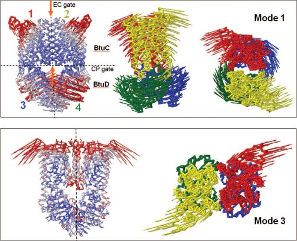
Global dynamics of the ABC transporter BtuCD. Top and bottom panels display the collective motions of the tetramer in the ANM modes 1 and 3, respectively, recently examined by Weng et al. (2008). The color-coded diagrams on the left in both panels display the size of motions (red, most mobile; blue, almost rigid) induced in these modes. The other diagrams display the relative motions of the two TM domains (1, red; 2, yellow) of the BtuC dimer, and the two NBDs (3, blue; 4, green) of the BtuD dimer, that compose the BtuCD tetramer, viewed from the side (middle diagram in top panel) or from the EC region (right diagrams in both panel). The two gates (EC and CP gates) of the substrate (vitamin B12) translocation pore are indicated by the orange arrows in the left diagram of the top panel.
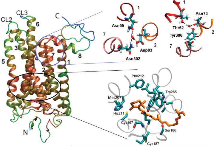
Critical interactions near the chromophore binding pocket and CP ends of TM1, TM2, and TM3 in rhodopsin. The ribbon diagram on the left is color-coded (from red, least mobile, to blue, most mobile) by the RMSDs observed in the positions of residues during ANM-steered MD simulations of rhodopsin activation. Two regions enlarged on the right are distinguished by their highly constrained dynamics: the chromophore binding pocket and the CP end of helices 1, 2, and 7. The tight packing in the former region ensures efficient propagation of the local conformational strains (induced upon cis → trans isomerization of the retinal) to distant regions, including in particular the ERY-binding motif at the CP end of helices H3 and H6 (note the enhanced mobility at this region). Water molecules play an important role in stabilizing the CP ends of TM1, TM2, and TM7. For more details, see ref .
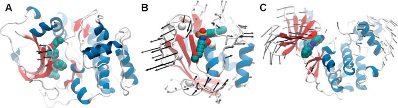
Use of NMA in modeling protein–ligand interactions. Alternative conformations for the target protein were generated for (A) cAMP-dependent protein kinase (PDB ID, 1JLU; inhibitor PDB ID, 1REK), (B) matrix metalloproteinase-3 (PDB ID, 1UEA; inhibitor PDB ID, 1HY7), and (C) cyclin-dependent kinase 2 (complex PDB ID, 1G5S), by reconfiguring these target proteins along the global modes of motions indicated by the arrows. See text for details.
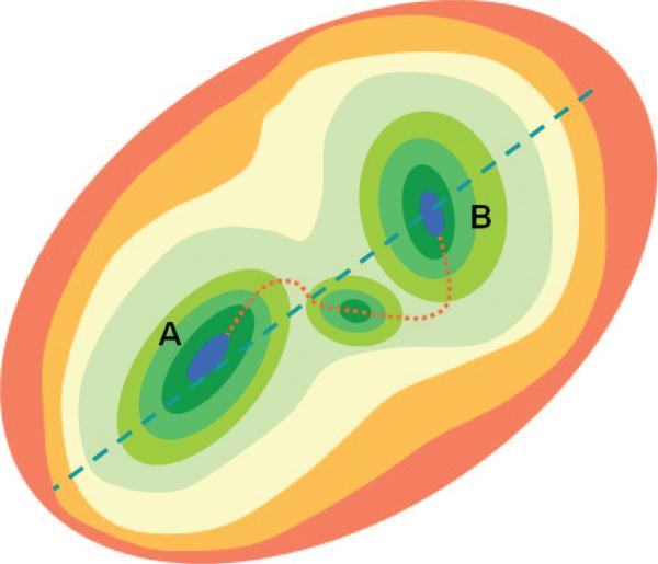
Schematic representation of the energy landscape for two substates. The cartoon shows the putative free energy landscape around a conformational transition for a two-state system. Both conformations, A and B, are contained within a global free energy well, represented here as the outermost oval. The slowest mode of the well, indicated by the broken blue line, is expected to overlap with the transition between states A and B. Each stable conformation lies at the bottom of its own local well. The transition between states (red dotted line) is expected to proceed along the slowest local mode in the vicinity of each end point. The slow modes accessible to the metastable intermediate conformation between the end points provide further information on the pathway near the transition point.
References
-
- Birshtein TM, Ptitsyn OB. Conformations of Macromolecules. Interscience; New York: 1966.
-
- Flory PJ. Statistical Mechanics of Chain Molecules. Wiley, Interscience (2nd Edition published in 1989 by Butterworth-Heinemann Ltd); New York: 1969. pp. 1–432.
-
- Volkenstein MV. Configurational Statistics of Polymer Chains. Interscience; New York: 1963.
-
- Taketomi H, Ueda Y, Go N. Int. J. Pept. Protein Res. 1975;7:445. - PubMed
-
- Noguti T, Go N, Ooi T, Nishikawa K. Biochim. Biophys. Acta. 1981;671:93. - PubMed
Publication types
MeSH terms
Substances
Grants and funding
LinkOut - more resources
Full Text Sources
