

Transforming Boolean models to continuous models: methodology and application to T-cell receptor signaling
- PMID: 19785753
- PMCID: PMC2764636
- DOI: 10.1186/1752-0509-3-98
Transforming Boolean models to continuous models: methodology and application to T-cell receptor signaling
Abstract
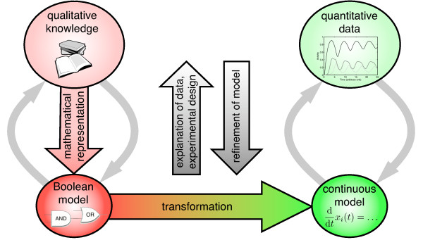
Background: The understanding of regulatory and signaling networks has long been a core objective in Systems Biology. Knowledge about these networks is mainly of qualitative nature, which allows the construction of Boolean models, where the state of a component is either 'off' or 'on'. While often able to capture the essential behavior of a network, these models can never reproduce detailed time courses of concentration levels. Nowadays however, experiments yield more and more quantitative data. An obvious question therefore is how qualitative models can be used to explain and predict the outcome of these experiments.
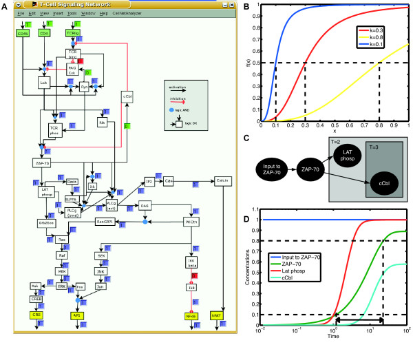
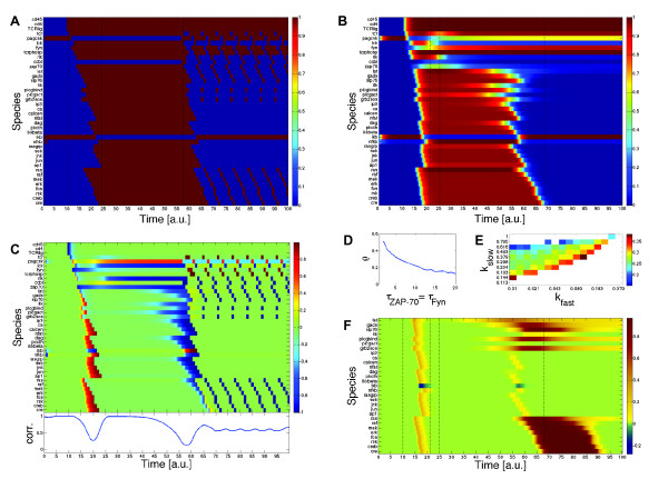
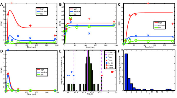
Results: In this contribution we present a canonical way of transforming Boolean into continuous models, where the use of multivariate polynomial interpolation allows transformation of logic operations into a system of ordinary differential equations (ODE). The method is standardized and can readily be applied to large networks. Other, more limited approaches to this task are briefly reviewed and compared. Moreover, we discuss and generalize existing theoretical results on the relation between Boolean and continuous models. As a test case a logical model is transformed into an extensive continuous ODE model describing the activation of T-cells. We discuss how parameters for this model can be determined such that quantitative experimental results are explained and predicted, including time-courses for multiple ligand concentrations and binding affinities of different ligands. This shows that from the continuous model we may obtain biological insights not evident from the discrete one.
Conclusion: The presented approach will facilitate the interaction between modeling and experiments. Moreover, it provides a straightforward way to apply quantitative analysis methods to qualitatively described systems.
Figures
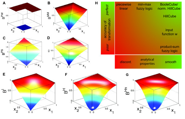
 . (B) Function
  obtained by min-max fuzzy logic and linear DOM functions. (C) Function
  obtained by product-sum fuzzy logic and linear DOM functions. (D) Input function ω introduced by Mendoza et al. [10]. (E) BooleCube
  obtained by multivariate polynomial interpolation. (F) HillCube
  . (G) normalized HillCube
  . In the last two figures parameters n = 3 and k = 0.5 were chosen for both inputs. (H) Overview of the different transformation techniques with respect to their analytical properties and transformation accuracy.
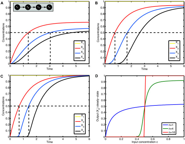
 = c > 0,
  = 0,
= 0,  = 0,
= 0,  = 0, for some constant input concentration c. The input node X1 remains constant and the other concentrations
  change accordingly to the ODE
  , i = 2, 3, 4. We simulate the model for different Hill coefficients n = 1, 4, 16 and input level c = 1; the results are shown in (A), (B) and (C). All three time courses show qualitatively the same cascade-like pattern. With growing n, however, the onset of activation of X3 and X4 comes closer and closer to the time point at which their activators X2 and X3, respectively, cross the threshold k. (D) shows the input-output curve. Plotted is the (constant) input concentration c of node X1 against the steady-state concentration of node X4. For n > 1, we observe the typical sigmoid stimulus-response behavior of signaling cascades, see e.g. [28]. With increasing n the steepness of the input-output curve increases, leading to an almost discrete (Boolean) output in the case n = 16.
References
Publication types
MeSH terms
Substances
Grants and funding
LinkOut - more resources
Full Text Sources
Research Materials
