Resolving the impact of waiting time distributions on the persistence of measles

Abstract

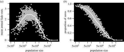
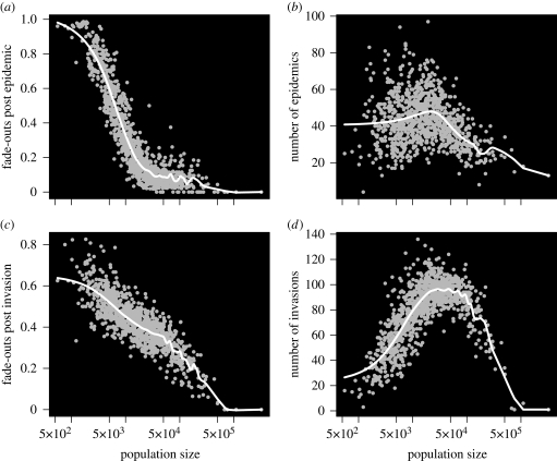
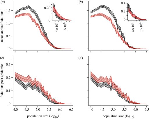
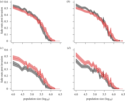
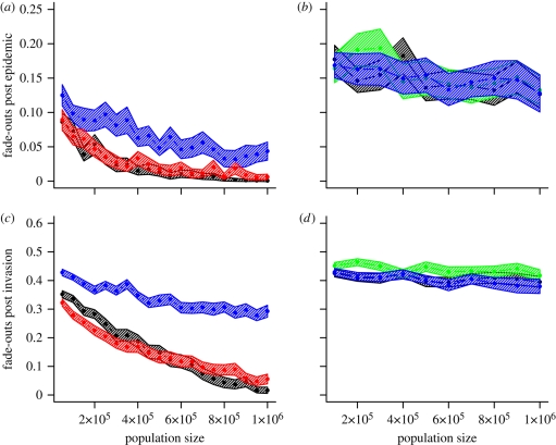
Measles epidemics in human populations exhibit what is perhaps the best empirically characterized, and certainly the most studied, stochastic persistence threshold in population biology. A critical community size (CCS) of around 250,000-500,000 separates populations where measles is predominantly persistent from smaller communities where there are frequent extinctions of measles between major epidemics. The fundamental mechanisms contributing to this pattern of persistence, which are long-lasting immunity to re-infection, recruitment of susceptibles, seasonality in transmission, age dependence of transmission and the spatial coupling between communities, have all been quantified and, to a greater or lesser level of success, captured by theoretical models. Despite these successes there has not been a consensus over whether simple models can successfully predict the value of the CCS, or indeed which mechanisms determine the persistence of measles over a broader range of population sizes. Specifically, the level of the CCS has been thought to be particularly sensitive to the detailed stochastic dynamics generated by the waiting time distribution (WTD) in the infectious and latent periods. We show that the relative patterns of persistence between models with different WTDs are highly sensitive to the criterion of comparison-in particular, the statistical measure of persistence that is employed. To this end, we introduce two new statistical measures of persistence-fade-outs post epidemic and fade-outs post invasion. Contrary to previous reports, we demonstrate that, no matter the choice of persistence measure, appropriately parametrized models of measles demonstrate similar predictions for the level of the CCS.

Figure 1.

Fade-out statistics for measles in England and Wales. Fade-out statistics for the 954 urban districts of England and Wales (1940–1964) are plotted in grey, with a smooth spline trend line overlaid in white. Population size of a district is taken to be the median population size over the period. (a) Mean annual fade-outs of measles (defined as 3 or more weeks with no reported cases) against population size. (b) Proportion of zero reports—the proportion of weeks with no reported cases of measles.

Figure 2.

Alternative fade-out statistics for measles in England and Wales. Fade-out statistics for the 954 urban districts of England and Wales (1940–1964) are plotted in grey, with a smooth spline trend line overlaid in white. Population size of a district is taken to be the median population size over the period. (a) Fade-outs post epidemic—number of fade-outs, defined as 3 or more weeks with no reported cases, divided by the number of epidemics over the period. (b) Number of epidemics—an epidemic is counted when the number of weekly reported cases falls below a (per capita) threshold value (T) of cases after previously rising above the same threshold; here we choose T = 1/2000 per capita. (c) Fade-outs post invasion—number of fade-outs, defined as 3 or more weeks with no reported cases, divided by the number of invasions over the period. (d) Number of invasions—an invasion is counted when the number of weekly reported cases crosses an absolute threshold (T) after a week with zero reports; here we choose T = 1.

Figure 3.

Interaction between seasonal forcing and the WTD. (a) The individual reproductive ratio for a term-time forcing function (R₀ = 17.0, α = 0.17) resulting from gamma-distributed WTDs in the latent and infectious stages with shape parameters κ_E = κ_I = κ. Dates of school terms are quoted in the electronic supplementary material. Black line, κ = 1; blue line, κ = 2; red line, κ = 5; green line, κ = 20. (b) The individual reproductive ratio for a cosine forcing function (R₀ = 17.0, α = 0.17) resulting from gamma-distributed WTDs in the latent and infectious stages with shape parameters κ_E = κ_I = κ. (c) Detail on the response of the individual reproductive ratio to the autumn half-term holiday. Parameters as in (a). (d) The individual reproductive ratio calculated for the trajectory-matched model fits from Keeling & Grenfell (2002). Transmission rates are reproduced in the electronic supplementary material (table a). Black lines are the two models with exponential WTDs (κ_E = κ_I = 1), red lines the two gamma (8,5) models (with κ_E = 8, κ_I = 5).

Figure 4.

Persistence in the simple model: mean annual fade-outs and fade-outs post epidemic. (a,b) Ensemble average (over 100 replicates of 24 years) of mean annual fade-outs against (log₁₀) population size for exponential (black) and the gamma (8,5) (red) models based on the comparison criteria of (a) constant parameters and (b) trajectory matching. Inset plots based on same simulated data, showing detail for large populations. (c,d) Ensemble average (over 100 replicates of 24 years) of fade-outs post epidemic (T = 1/2000 per capita) against (log₁₀) population size for exponential (black) and the gamma (8,5) (red) models based on the comparison criteria of (c) constant parameters and (d) trajectory matching. Parameter values as described in the main text. Shaded envelope represents a 95 per cent confidence interval calculated as 1.96 standard errors, based on 100 replicates of 24 years. Imports of infection are scaled with the square root of population size (0.02√N imports per year).

Figure 5.

Persistence in the simple model: fade-outs post invasion. (a,b) Ensemble average (over 100 replicates of 24 years) of fade-outs post invasion against (log₁₀) population size for exponential (black) and the gamma (8,5) (red) models based on the comparison criteria of (a) constant parameters and (b) trajectory matching with threshold T = 1. (c,d) Ensemble average (over 100 replicates of 24 years) of fade-outs post invasion against (log₁₀) population size for exponential (black) and the gamma (8,5) (red) models based on the comparison criteria of (c) constant parameters and (d) trajectory matching with threshold T = 5. Parameter values as described in the main text. Shaded envelope represents a 95 per cent confidence interval calculated as 1.96 standard errors, based on 100 replicates of 24 years. Imports of infection are scaled with the square root of population size (0.02√N imports per year).

Figure 6.

Static age distributions under cohort and fractional ageing. The predicted susceptible proportion, before and after ageing, in infants (0–5), primary school children (5–10), adolescents (10–20) and adults (20+) under (a) fractional ageing and (b) cohort ageing. Proportions are calculated based on the form of the force of infection assumed by the PRAS model. Details of this calculation can be found in the electronic supplementary material (§3). Blue rectangle, start of year; red rectangle, end of year.

Figure 7.

Persistence in age-structured models: fractional versus cohort ageing. PRAS, Bolker and Babad models use transmission parameters estimated by Keeling & Grenfell (1997), Bolker & Grenfell (1995) and Babad et al. (1994), respectively. The shape parameters used for the (gamma distributed) infectious and latent periods for each model are indicated by parentheses (κ_E, κ_I). (a,b) Ensemble average (over 100 replicates of 24 years) of fade-outs post epidemic against population size for (a) fractional and (b) cohort ageing (T = 1/2000 per capita). (c,d) Ensemble average (over 100 replicates of 24 years) of fade-outs post invasion against population size for (c) fractional and (d) cohort ageing (T = 1). Shaded envelope represents a 95 per cent confidence interval calculated as 1.96 standard errors, based on 100 replicates of 24 years. Imports of infection are fixed (independent of population size) at 10 infectious imports per year. Black line, PRAS (1,1); red line, PRAS (8,5); blue line, Bolker (1,1); green line, Babad (1,1).

References

-
- Anderson D., Watson R. 1980. On the spread of a disease with gamma distributed latent and infectious periods. Biometrika 67, 191–198. (10.1093/biomet/67.1.191) - DOI
- Anderson R. M., May R. M. 1991. Infectious diseases of humans: dynamics and control. New York, NY: Oxford University Press.
Publication types
MeSH terms
Grants and funding
LinkOut - more resources
Full Text Sources