Contrast sensitivity in natural scenes depends on edge as well as spatial frequency structure

Abstract

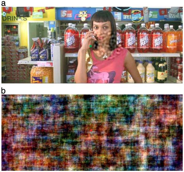
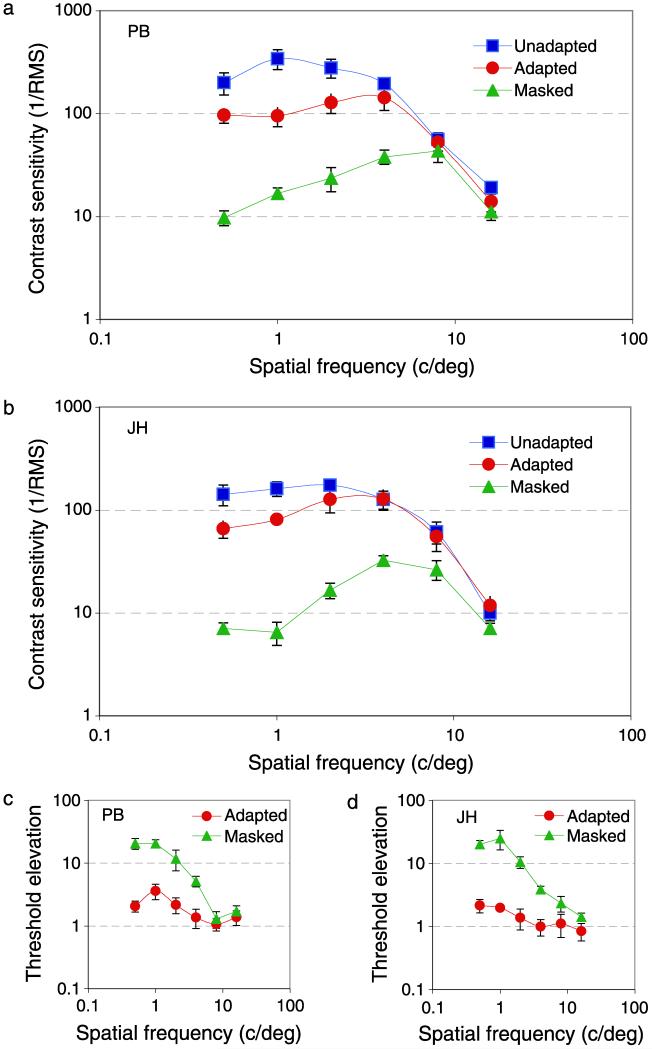
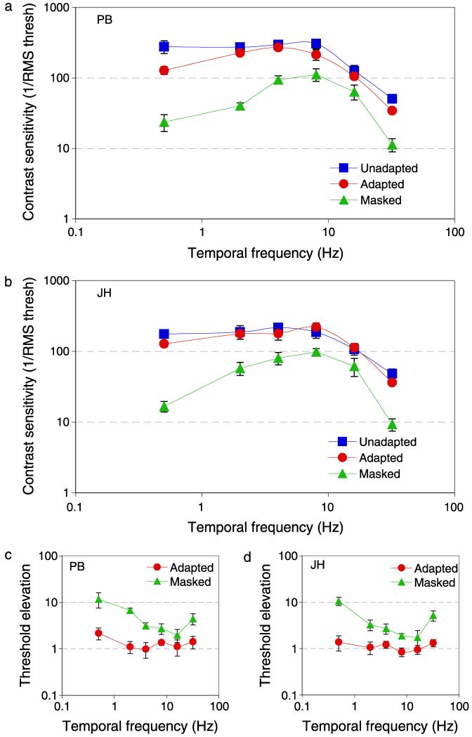
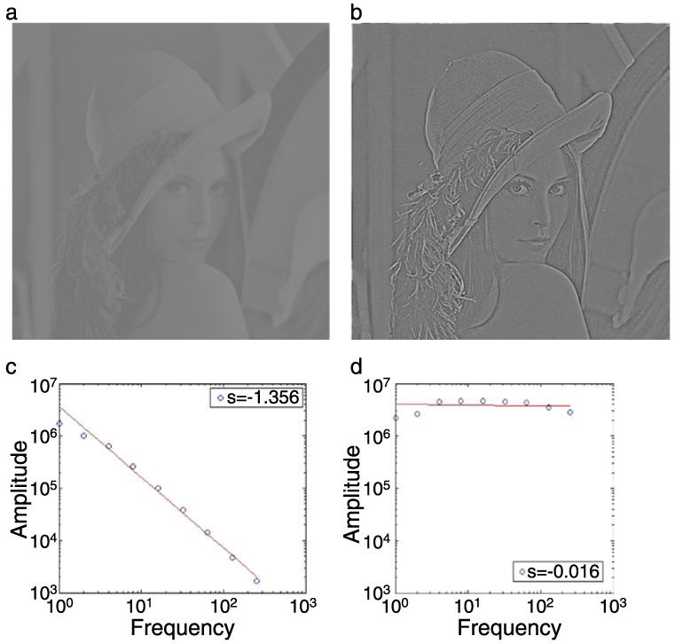
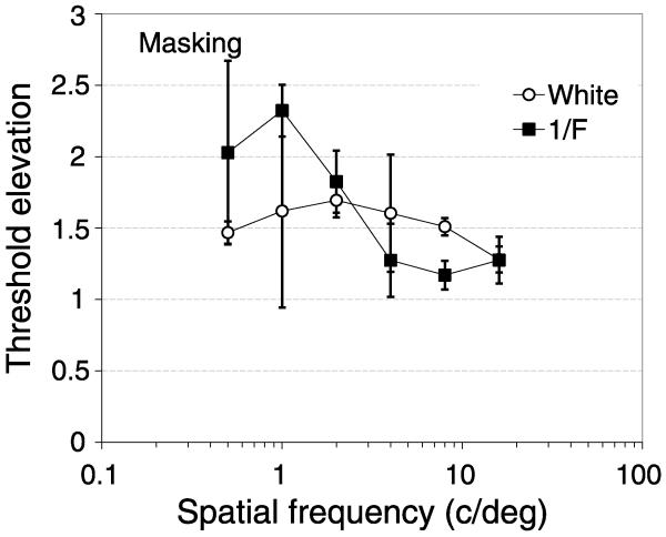
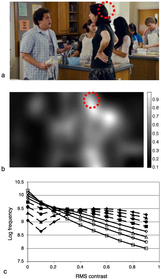
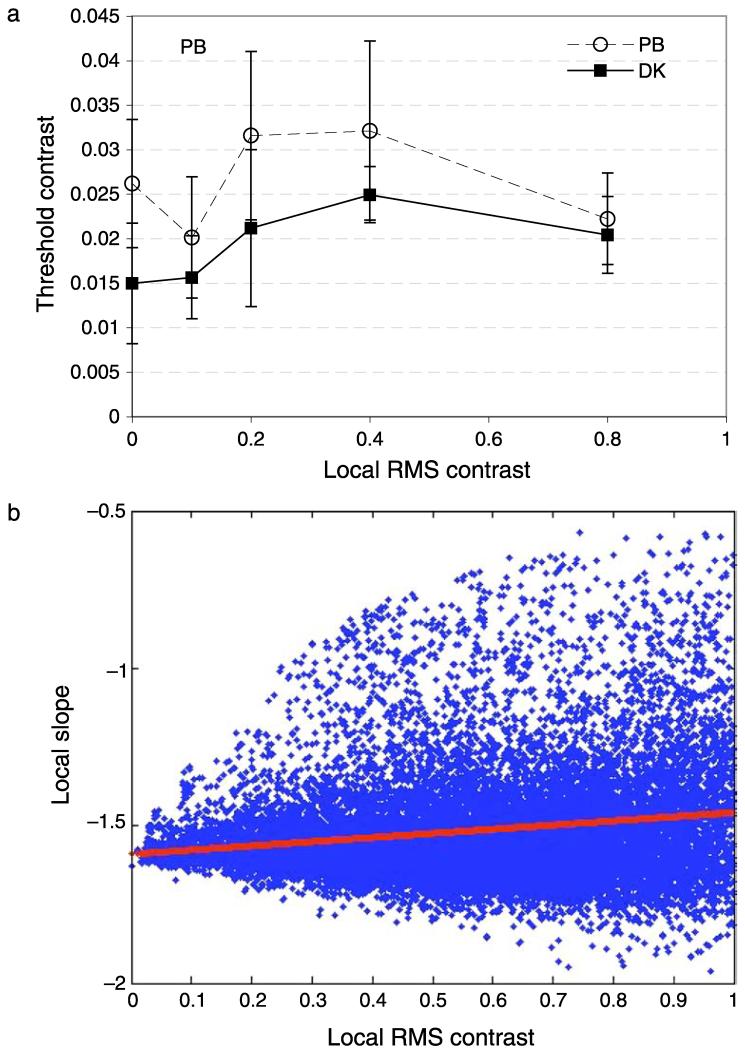
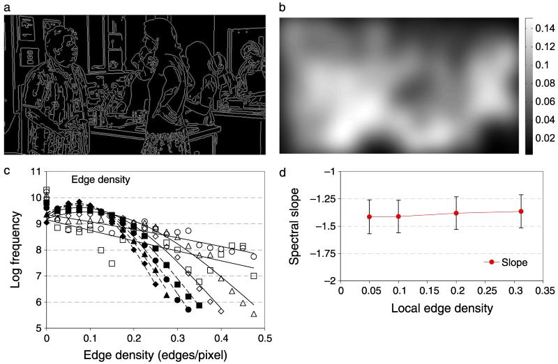
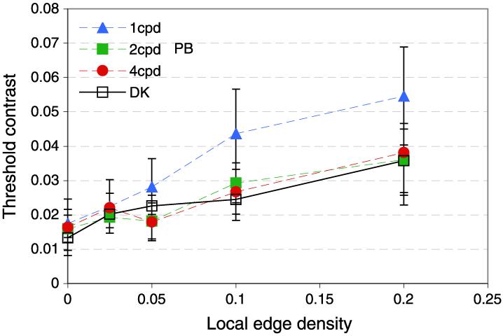
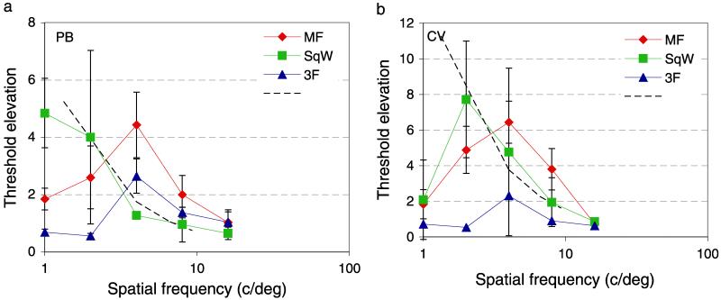
The contrast sensitivity function is routinely measured in the laboratory with sine-wave gratings presented on homogenous gray backgrounds; natural images are instead composed of a broad range of spatial and temporal structures. In order to extend channel-based models of visual processing to more natural conditions, we examined how contrast sensitivity varies with the context in which it is measured. We report that contrast sensitivity is quite different under laboratory than natural viewing conditions: adaptation or masking with natural scenes attenuates contrast sensitivity at low spatial and temporal frequencies. Expressed another way, viewing stimuli presented on homogenous screens overcomes chronic adaptation to the natural environment and causes a sharp, unnatural increase in sensitivity to low spatial and temporal frequencies. Consequently, the standard contrast sensitivity function is a poor indicator of sensitivity to structure in natural scenes. The magnitude of masking by natural scenes is relatively independent of local contrast but depends strongly on the density of edges even though neither greatly affects the local amplitude spectrum. These results suggest that sensitivity to spatial structure in natural scenes depends on the distribution of local edges as well as the local amplitude spectrum.

Figure 1

Illustrations of the stimuli. (a) A single frame from a movie. This image contains a band-pass-filtered noise target to the right of fixation that was present in only the masking condition (see text for details). (b) Random phase version of (a) in which the same random phase offset has been applied in each RGB plane to preserve the chromatic properties of the original image. The green and red circles show isoluminant fixation points whose color indicated whether the observer’s response was correct or incorrect.

Figure 2

(a, b) Spatial frequency contrast sensitivity and (c, d) threshold elevations for two observers (PB and JH). Blue squares show standard contrast sensitivity (in which targets were presented on mean luminance backgrounds), red circles show data from adapted conditions (in which a movie was played for at least 5 s between test periods), and green triangles show data for the masking condition (where the target was presented within a real movie). The x-axis shows the peak spatial frequency of the band-pass-filtered noise target, the y-axis shows contrast sensitivity, defined as the inverse of the rms contrast required for correct detection of the target on 75% trials. Threshold elevations are relative to standard (blue data) conditions. Error bars show ±95% confidence intervals on all figures.

Figure 3

(a, b) Temporal frequency contrast sensitivity and (c, d) threshold elevations for two observers (PB and JH). As Figure 2 except for temporal frequency.

Figure 4

Illustration of spatial whitening. (a) A natural image whose amplitude spectrum, plotted in (c), falls approximately as “1/F” on log–log axes with a slope of −1.4. Whitening the amplitude spectrum produces an image (b) that appears sharpened, but otherwise structurally quite similar. (d) The amplitude spectrum of the whitened image has approximately the same amplitude at all spatial frequencies and a resultant spectral slope close to 0. The rms contrasts of the source and whitened images have been fixed at 0.25.

Figure 5

Threshold elevations (masked divided by unmasked contrast threshold) for band-pass-filtered targets presented in 1/F (filled symbols) or spatially whitened (open symbols) movies. Data show the mean results for three subjects for standard grayscale (filled squares) or whitened (open circles) movies. Error bars show ±95% confidence intervals.

Figure 6

Illustration of local contrast estimation. (a) A typical frame from one of our movies. A Gaussian weighted function was used to compute the local mean luminance and local standard deviation that were used to estimate local rms contrast. (b) Local rms contrast computed this way for (a). The gray level of each pixel corresponds to the local contrast at that point, see scale bar. (c) The distribution of rms contrast in 75,000 movie frames. The standard deviation of the Gaussian was 720 pixels (1 cycle/image, filled diamonds), 360 (filled triangles), 180 (filled circles), 90 (filled squares), 45 (open diamonds), 22.5 (open triangles), 11.25 (open circles), or 5.125 (open squares).

Figure 7

(a) Contrast detection as a function of local rms contrast for two observers. The target was band-pass-filtered noise with 2 c/deg peak spatial frequency and 2.4-Hz peak temporal frequency, presented within a Gaussian spatio-temporal envelope. The x-axis shows the local rms contrast at the test location (see text for explanation). Error bars show 95% confidence intervals. (b) Scatter plot of the slope of the local amplitude spectrum as a function of local rms contrast (blue data). Red data show the best straight line fit.

Figure 8

Illustration of local edge density estimation. The edges of each movie frame were determined by a Canny edge-finding algorithm. (a) The edges identified in Figure 4a. (b) A Gaussian weighted function was used to compute the local edge density (proportion of edge pixels) over the target area, shown by the scale bar. (c) The distribution of edge densities across 75,000 movies. The standard deviation of the Gaussian was 720 pixels (1 cycle/image, filled diamonds), 360 (filled triangles), 180 (filled circles), 90 (filled squares), 45 (open diamonds), 22.5 (open triangles), 11.25 (open circles), or 5.125 (open squares). High edge density regions are not common in natural scenes. Most areas have fewer than 0.2 edges per pixel. The effect of edge density on the slope of the amplitude spectrum (d) is small and there is significant overlap in the slopes at all edge densities tested.

Figure 9

Edge density in natural scenes. (a) Frequency distribution of local edge density contrast over 2.68 × 10¹⁰ pixels. (b) Contrast detection as a function of local edge density for two observers (PB, filled symbols and DK, open squares). The target was band-pass-filtered noise pattern with peak spatial frequency at 1 c/deg (triangles), 2 c/deg (squares), or 4 c/deg (circles) and 2.4-Hz peak temporal frequency, presented within a Gaussian spatio-temporal envelope. The x-axis shows the local edge density at the test location (see text for explanation). Error bars show 95% confidence intervals.

Figure 10

Contrast threshold elevations for sine grating targets presented with masking waveforms for two observers (PB and CV). The target was a horizontal Gabor patch with fixed spatial (2 deg) and temporal (107 ms) standard deviation and spatial frequency from 1 to 16 c/deg in log steps. Masks were presented within the same Gaussian spatio-temporal envelope and was either a 1.3 c/deg square grating of 25% Michelson contrast (green squares), a 1.3 c/deg missing fundamental grating of 0.25 contrast (red circles), or a 4 c/deg Gabor of 8.3% contrast (blue triangles). Dashed line shows the expected loss in sensitivity for a square-wave grating.

References

1. Atick JJ. Could information theory provide an ecological theory of sensory processing? Network: Computation in Neural Systems. 1992;3:213–251. - PubMed
1. Balboa RM, Grzywacz NM. Occlusions and their relationship with the distribution of contrasts in natural images. Vision Research. 2000;40:2661–2669. PubMed. - PubMed
1. Balboa RM, Grzywacz NM. Power spectra and distribution of contrasts of natural images from different habitats. Vision Research. 2003;43:2527–2537. PubMed. - PubMed
1. Barlow HB. Possible principles underlying the transformation of sensory messages. In: Rosenblith WA, editor. Sensory communication. MIT Press; Cambridge, MA: 1961. pp. 217–234.
1. Betsch BY, Einhäuser W, Körding KP, König P. The world from a cat’s perspective—Statistics of natural videos. Biological Cybernetics. 2004;90:41–50. PubMed. - PubMed
Publication types