A genealogical interpretation of principal components analysis
- PMID: 19834557
- PMCID: PMC2757795
- DOI: 10.1371/journal.pgen.1000686
A genealogical interpretation of principal components analysis
Abstract
Principal components analysis, PCA, is a statistical method commonly used in population genetics to identify structure in the distribution of genetic variation across geographical location and ethnic background. However, while the method is often used to inform about historical demographic processes, little is known about the relationship between fundamental demographic parameters and the projection of samples onto the primary axes. Here I show that for SNP data the projection of samples onto the principal components can be obtained directly from considering the average coalescent times between pairs of haploid genomes. The result provides a framework for interpreting PCA projections in terms of underlying processes, including migration, geographical isolation, and admixture. I also demonstrate a link between PCA and Wright's f(st) and show that SNP ascertainment has a largely simple and predictable effect on the projection of samples. Using examples from human genetics, I discuss the application of these results to empirical data and the implications for inference.
Conflict of interest statement
The author has declared that no competing interests exist.
Figures
 and
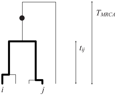
and  , will share a derived mutation (indicated by the circle) if it occurs on the branch between their most recent common ancestor and the common ancestor of the whole sample. The length of this branch is
  .
.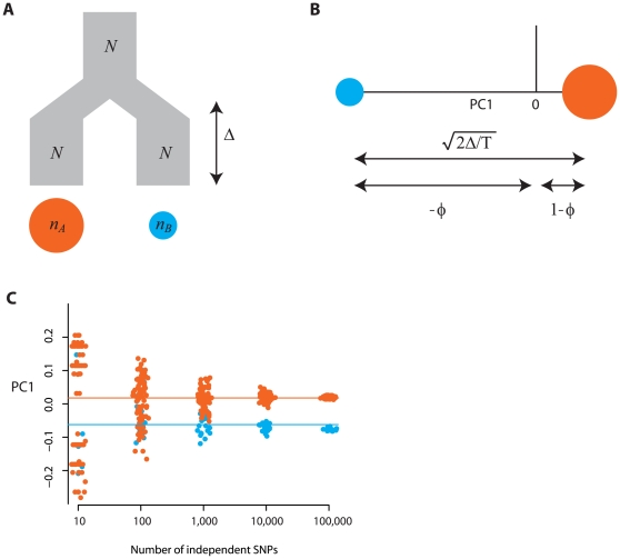
 individuals from population A (indicated by the red circle) and
  from population B (indicated by the blue circle), where the two populations have the same effective population size of
  and are both derived from a single ancestral population, also of size
  , with the split happening a time
  in the past. (B) The expected locations of these two sets of samples on the first PC is defined by the time since divergence (the Euclidean distance between the samples is
  ) (see text for definitions) and the relative sample size from the populations, with the larger sample lying closer to the origin. Defining
  , the relative location of the two populations on the first PC are
  for samples from population A and
  for samples from population B (note that the sign is arbitrary). (C) To investigate the effect of finite genome size simulations were carried out for the model shown in part A with 80 genomes sampled from population A, 20 from population B and a split time of 0.02
  generations (
 ) and between
  and
and  SNPs. Lines indicate the analytical expectation. A jitter has been added to the x-axis for clarity. Note that the separation of samples with 10 SNPs does not correlate with population and simply reflects random clustering arising from the small numbers of SNPs.
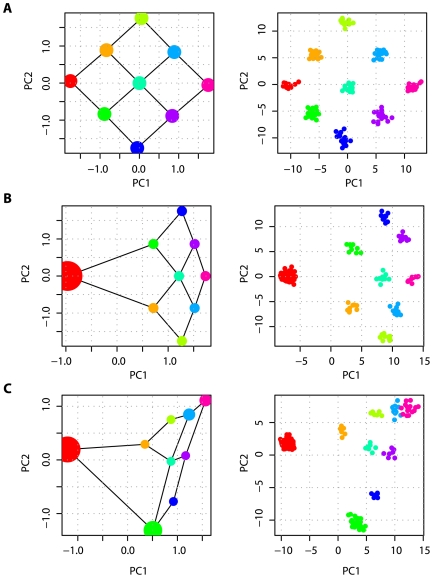
 per
per  generations with each adjoining neighbour, leads to a recovery of the migration-space if samples are of equal size (A), or a distortion of migration-space if populations are not equally represented (B,C). In each part the left-hand panel shows the analytical solution (the area of each point represents the relative sample size) with migration routes illustrated while the right-hand panel shows the result of a simulation with a total sample size of 180 and 10,000 independent SNP loci. All examples are for
  .
.
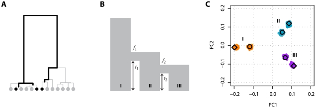
 ,
,  ,
,  ,
,  , where
  is the bottleneck strength measured as the probability that two lineages entering the bottleneck have coalesced by its end (the bottleneck is instantaneous in real time). All populations have the same effective population size. (C) PCA of the simulated data (small open circles) shows strong agreement with results obtained from analytical consideration of the expected coalescence times (large circles). When only those SNPs that have been discovered in a small panel are considered (here modelled as 4, 8, and 4 additional samples from populations I, II, and III respectively) the principal effect is to scale the locations of the samples on the first two PCs (small filled circles) by a factor of approximately
  (large diamonds).
References
-
- Patterson N, Price AL, Reich D. Population structure and eigenanalysis. PLoS Genet. 2006;2:e190. doi: 10.1371/journal.pgen.0020190. - DOI - PMC - PubMed
-
- Price AL, Patterson NJ, Plenge RM, Weinblatt ME, Shadick NA, et al. Principal components analysis corrects for stratification in genome-wide association studies. Nat Genet. 2006;38:904–909. - PubMed
-
- Cavalli-Sforza LL, Menozzi P, Piazza A. The History and Geography of Human Genes. New Jersey: Princeton; 1994.
-
- Reich D, Price AL, Patterson N. Principal component analysis of genetic data. Nat Genet. 2008;40:491–492. - PubMed
Publication types
MeSH terms
LinkOut - more resources
Full Text Sources
Other Literature Sources
Miscellaneous