Spinal interneurons differentiate sequentially from those driving the fastest swimming movements in larval zebrafish to those driving the slowest ones

Abstract

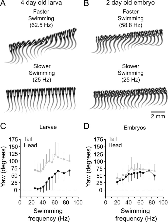
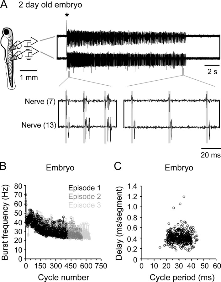
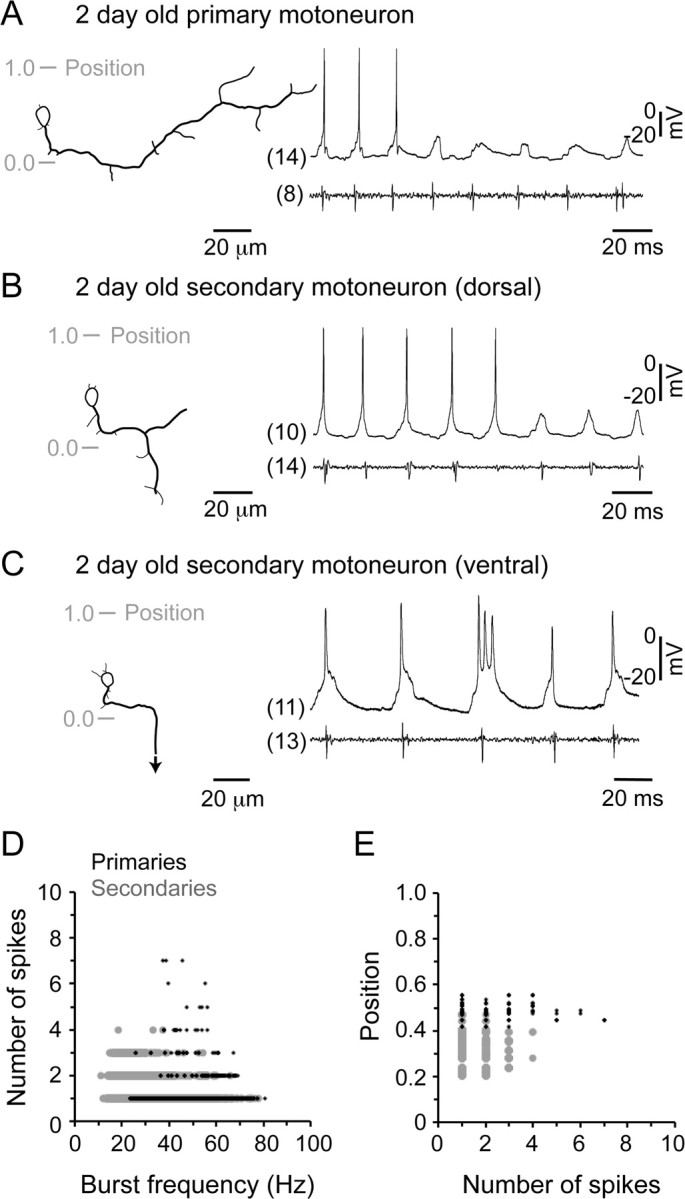
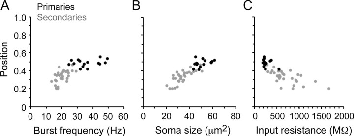
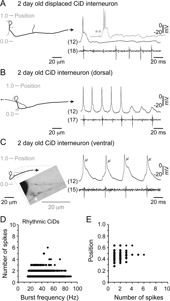
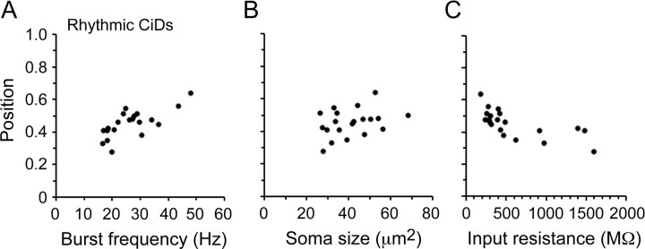
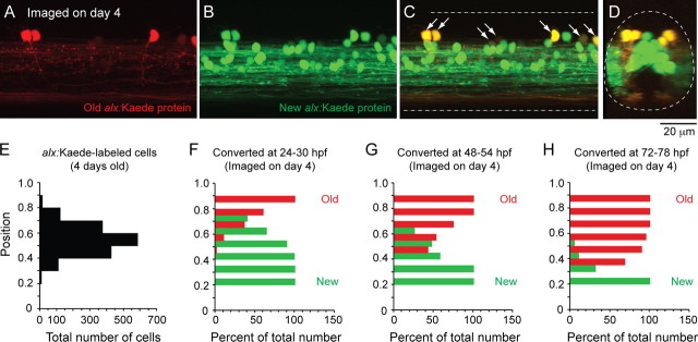
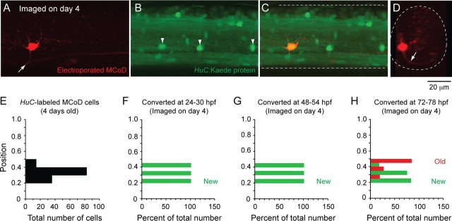
Studies of neuronal networks have revealed few general principles that link patterns of development with later functional roles. While investigating the neural control of movements, we recently discovered a topographic map in the spinal cord of larval zebrafish that relates the position of motoneurons and interneurons to their order of recruitment during swimming. Here, we show that the map reflects an orderly pattern of differentiation of neurons driving different movements. First, we use high-speed filming to show that large-amplitude swimming movements with bending along much of the body appear first, with smaller, regional swimming movements emerging later. Next, using whole-cell patch recordings, we demonstrate that the excitatory circuits that drive large-amplitude, fast swimming movements at larval stages are present and functional early on in embryos. Finally, we systematically assess the orderly emergence of spinal circuits according to swimming speed using transgenic fish expressing the photoconvertible protein Kaede to track neuronal differentiation in vivo. We conclude that a simple principle governs the development of spinal networks in which the neurons driving the fastest, most powerful swimming in larvae develop first with ones that drive increasingly weaker and slower larval movements layered on over time. Because the neurons are arranged by time of differentiation in the spinal cord, the result is a topographic map that represents the speed/strength of movements at which neurons are recruited and the temporal emergence of networks. This pattern may represent a general feature of neuronal network development throughout the brain and spinal cord.

Figure 1.

A, B, Kinematic analysis of swimming movements in zebrafish embryos and larvae. A, Successive, overlapping images captured at 1000 frames per second of a larval zebrafish swimming at ∼60 Hz (faster swimming, top) and 25 Hz (slower swimming, bottom). Top images are illustrated every millisecond, and at the bottom they are every 2 ms. B, Successive, overlapping images of an embryonic zebrafish swimming around 60 Hz (faster swimming, top) and around 25 Hz (slower swimming, bottom). As in A, top images are illustrated every millisecond, and at the bottom they are every 2 ms. White bars in A and B illustrate the lateral displacement, or yaw, of the head during swimming. C–D, Plots of larval (C) and embryonic (D) head (black circles) and tail (gray circles) yaw during various speeds of swimming. Data are binned and averaged every 5 Hz. Errors are SDs. These data are compiled from 25 episodes of stimulus-induced swimming from five embryos and 50 episodes of swimming (25 spontaneous, 25 stimulus-induced) from five larvae.

Figure 2.

Fictive swimming motor pattern in embryos. A, Schematic on the left illustrates the position from which motor nerve recordings illustrated on the right are taken (7th and 13th body segments). An electrical stimulus delivered to the tail was used to elicit swimming (artifact at asterisk). Top right, Single episode of swimming on a slower time base; bottom right, illustration, on a faster time base, of motor bursts that would drive cyclical bending. Transparent gray boxes illustrate the head-to-tail delay of motor bursts. B, Plot of motor nerve burst frequency (measured from the tail) with respect to the cycle in the episode from three electrically evoked episodes in the same embryo. C, Plot of head–tail motor burst delay versus cycle period in a single embryo. These data are compiled from one episode of electrical stimulus-induced swimming from one embryo. Correlation values: r = −0.08, p = 0.10, n = 406 cycles.

Figure 3.

Motoneuron firing during fictive swimming. A, Recording from a primary motoneuron in an embryo, with a reconstructed drawing of the cell on the left and the corresponding physiology immediately to the right. Gray-shaded lines indicate the position with respect to the dorsal (1.0) and ventral (0.0) edges of spinal cord. The respective segment from which the cell and the nerve recording were obtained is indicated in parentheses. B, Recording from a dorsally located secondary motoneuron is organized as detailed in A. C, Recording from a ventrally located secondary motoneuron is organized as detailed in A. An arrow indicates continuation of the axon out of the field of view. D, Plot of the number of spikes per cycle generated by motoneurons versus swimming frequency. Data represent 11,167 cycles from 30 secondary motoneurons (gray circles) and 1123 cycles from 15 primaries (black dots). E, Plot of the somatic dorsoventral position of motoneurons versus the number of spikes. Graphs are plotted from the same dataset in D.

Figure 4.

Motoneuron recruitment, size, and excitability in embryos. A, Plot of spinal cord position versus swimming frequency for 15 primary motoneuron somata (black circles) and 30 secondary motoneurons (gray circles). Correlation values: r = 0.28, p = 0.30, n = 15 (primaries), r = 0.56, p < 0.01, n = 30 (secondaries), r = 0.77, p < 0.0001, n = 45 (combined primaries and secondaries). B, Plot of soma position versus soma size for the same motoneurons in A. Correlation values: r = 0.36, p = 0.19, n = 15 (primaries), r = 0.76, p < 0.0001, n = 30 (secondaries), r = 0.87, p < 0.0001, n = 45 (combined). C, Plot of soma position versus input resistance for the same motoneurons in A and B. Correlation values: r = −0.32, p = 0.25, n = 15 (primaries), r = −0.64, p < 0.001, n = 30 (secondaries), r = −0.79, p < 0.0001, n = 45 (combined). Each data point in A–C represents the mean value for each cell.

Figure 5.

Excitatory interneuron firing during fictive swimming. A, Recording from a dorsally displaced CiD interneuron in an embryo, with the reconstructed cells on the left and the corresponding physiology immediately to the right. Gray-shaded lines indicate the position with respect to the dorsal (1.0) and ventral (0.0) edges of spinal cord. The arrow indicates continuation of the axon out of the field of view. The respective segment from which the cell and the nerve recording were obtained is indicated in parentheses. The gray-shaded trace inset is from the same CiD cell and illustrates only the patch recording in response to a suprathreshold stimulus (double asterisk). While the stronger stimulus could not elicit firing in consecutive cycles, it did, however, cause more spikes. B, Recording from a dorsally located CiD interneuron is organized as detailed for A. Note the prominent ascending axon. C, Recording from a ventrally located CiD interneuron is organized as detailed for A. A photograph detailing the boxed region of the cell is inset, and a white arrow points out the growth of what is most likely new axon. Gray arrows point out the relatively broad action potentials of this cell. D, Plot of the number of spikes per cycle generated by excitatory interneurons versus swimming frequency. Data represent 12,641 cycles from 20 CiD cells (black circles). E, Plot of the somatic dorsoventral position of excitatory interneurons versus the number of spikes. Graph is plotted from the same dataset in D.

Figure 6.

Excitatory interneuron recruitment, size, and excitability in embryos. A, Plot of spinal cord position versus swimming frequency for 20 CiD somata (open black circles). Correlation values: r = 0.72, p < 0.001, n = 20. B, Plot of soma position versus soma size for the same CiDs in A. Correlation values: r = 0.34, p = 0.15, n = 20. C, Plot of soma position versus input resistance for the same CiDs in A and B. Correlation values: r = −0.68, p < 0.001, n = 20. Each data point in A–C represents the mean value for each cell.

Figure 7.

Kaede labeling to track alx-labeled CiD interneuron differentiation in vivo. A–C, Confocal z stack (54 μm in depth) from midbody (segment 15) illustrates alx cells labeled with the photoconvertible protein Kaede in a 4-d-old larva. Cells expressing Kaede at the time of photoconversion (24–30 hpf or 1 d old) contain red labeling at day 4 (A), while those that differentiated after day 1 have only green labeling (B). A merged image demonstrates that older, red cells continued to express new, green Kaede protein and so are yellow (at arrows) (C). D, An optical cross section of the z stack in A–C illustrates that older cells are more dorsally and laterally located. E, A bar chart illustrating the dorsoventral distribution of all 1620 alx:Kaede-labeled cells from 21 larvae. F–H, Bar charts illustrating the percentage of alx:Kaede-labeled cells imaged on day 4 at different dorsoventral locations that contained any red Kaede protein (old, red bars) or only green Kaede protein (new, green bars) when converted at either 24–30 hpf (day 1, F), 48–54 hpf (day 2, G), or 72–78 hpf (day 3, H).

Figure 8.

Kaede labeling to track MCoD differentiation in vivo. A–C, Confocal z stack (47 μm in depth) from midbody (segment 15) illustrates an MCoD electroporated with dye in a 4-d-old transgenic HuC:Kaede fish. A, The MCoD axon crosses spinal cord at the white arrow. B, White arrowheads mark laterally located cells, which are likely MCoDs. C, Merged image demonstrates one of the laterally located HuC:Kaede cells is indeed an MCoD and so is yellow. D, An optical cross section of the z stack in A illustrates that the MCoD is located ventrally and has a commissural process (at white arrow). E, A bar chart illustrating the dorsoventral distribution of all 131 HuC:Kaede-labeled MCoD cells from 32 4-d-old larvae. F–H, Bar charts illustrating the percentage of HuC:Kaede-labeled MCoD cells imaged on day 4 at different dorsoventral locations that contained any red Kaede protein (old, red bars) or only green Kaede protein (new, green bars) when converted at either 24–30 hpf (day 1, F), 48–54 hpf (day 2, G), or 72–78 hpf (day 3, H).

References

1. Altman J, Bayer SA. Development of the brain stem in the rat. IV. Thymidine-radiographic study of the time of origin of neurons in the pontine region. J Comp Neurol. 1980;194:905–929. - PubMed
1. Angevine JB, Jr, Sidman RL. Autoradiographic study of cell migration during histogenesis of cerebral cortex in the mouse. Nature. 1961;192:766–768. - PubMed
1. Beattie CE, Hatta K, Halpern ME, Liu H, Eisen JS, Kimmel CB. Temporal separation in the specification of primary and secondary motoneurons in zebrafish. Dev Biol. 1997;187:171–182. - PubMed
1. Bekoff A, Trainer W. The development of interlimb co-ordination during swimming in postnatal rats. J Exp Biol. 1979;83:1–11. - PubMed
1. Berkowitz A. Physiology and morphology of shared and specialized spinal interneurons for locomotion and scratching. J Neurophysiol. 2008;99:2887–2901. - PubMed
Publication types
MeSH terms
Substances
LinkOut - more resources