Specific entrainment of mitral cells during gamma oscillation in the rat olfactory bulb

Abstract

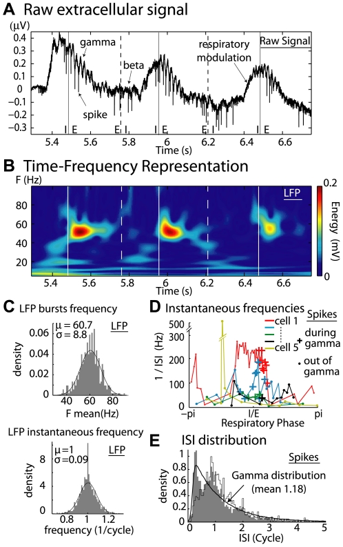
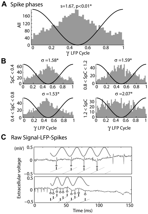
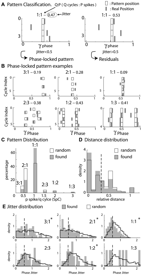
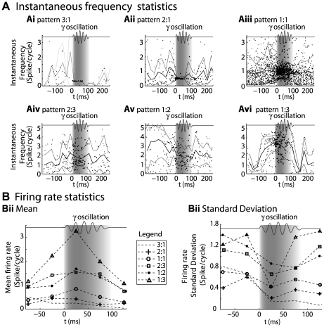
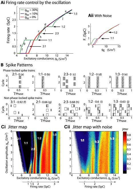
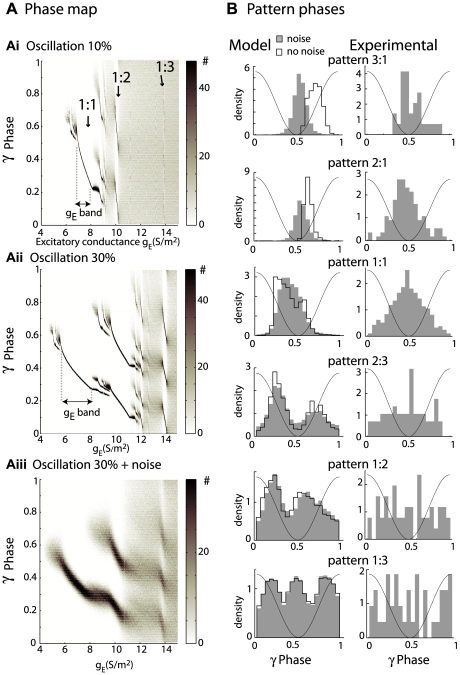
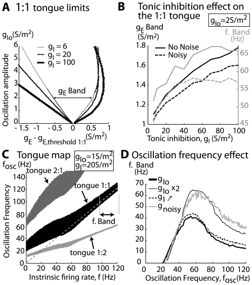
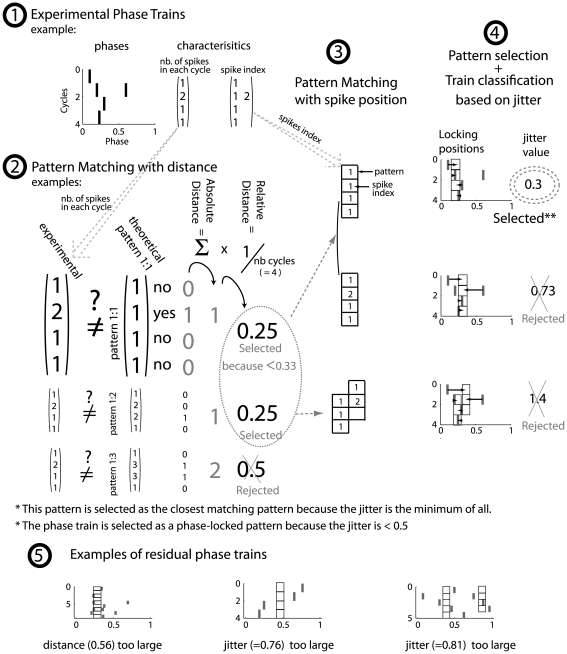
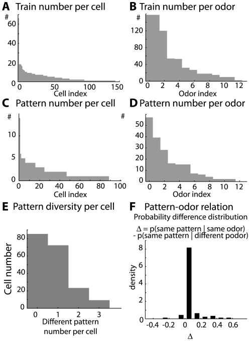
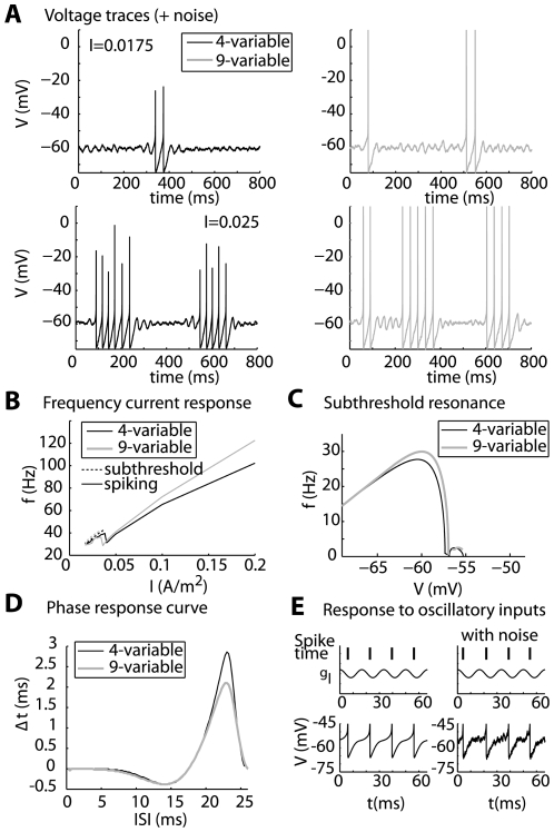
Local field potential (LFP) oscillations are often accompanied by synchronization of activity within a widespread cerebral area. Thus, the LFP and neuronal coherence appear to be the result of a common mechanism that underlies neuronal assembly formation. We used the olfactory bulb as a model to investigate: (1) the extent to which unitary dynamics and LFP oscillations can be correlated and (2) the precision with which a model of the hypothesized underlying mechanisms can accurately explain the experimental data. For this purpose, we analyzed simultaneous recordings of mitral cell (MC) activity and LFPs in anesthetized and freely breathing rats in response to odorant stimulation. Spike trains were found to be phase-locked to the gamma oscillation at specific firing rates and to form odor-specific temporal patterns. The use of a conductance-based MC model driven by an approximately balanced excitatory-inhibitory input conductance and a relatively small inhibitory conductance that oscillated at the gamma frequency allowed us to provide one explanation of the experimental data via a mode-locking mechanism. This work sheds light on the way network and intrinsic MC properties participate in the locking of MCs to the gamma oscillation in a realistic physiological context and may result in a particular time-locked assembly. Finally, we discuss how a self-synchronization process with such entrainment properties can explain, under experimental conditions: (1) why the gamma bursts emerge transiently with a maximal amplitude position relative to the stimulus time course; (2) why the oscillations are prominent at a specific gamma frequency; and (3) why the oscillation amplitude depends on specific stimulus properties. We also discuss information processing and functional consequences derived from this mechanism.

Figure 1. Unit activities and LFP gamma oscillation frequencies had the same mean but very different variability.

A) Raw signal recorded in the MC layer during odorant stimulation. Vertical continuous lines: I/E transitions; vertical dashed lines: E/I transitions. B) Time frequency representation extracted from the raw signal and based upon a wavelet transformation. The signal energy at each time-frequency point is in a colorscale. C) Top) Distribution of LFP gamma-burst mean frequencies with a normal function fit, which is shown as a black trace. Bottom) Distribution of LFP cycle instantaneous frequency, which is defined as the inverse of the period between two max of the oscillation, and which is normalized to the average frequency of the gamma burst to which the cycle belongs. D) Instantaneous frequencies along one respiratory cycle (six colors for six cells). + are spike positions for which gamma LFP oscillations are present. E) Interspike interval distribution (ISI) for spike trains occurring during gamma oscillations (bin 0.05 cycle, black line, gamma function distribution with the same mean ISI as the experimentally found (see methods)). Contour histogram is the distribution of the mean ISIs that was calculated for each spike train. All units are given in “cycle”.

Figure 2. Rate dependence of spike phase distribution during gamma oscillation.

A) Spike phase distribution (phase bin = 0.02 cycle) for all spikes during gamma oscillation (black line). The coupling strength was weak and statistically significant [mean = 0.472, average length, r = 0.25, circular deviation = 1.67; p<0.01, Rayleigh test)]. B) Spike phase distribution according to the mean spike rate (measured in Spike per Cycle (SpC)), (see y-label). (* indicate p<0.01 for a non-homogeneous distribution). The phase means were 0.480, 0.471, 0.486, 0.409, phase average lengths were 0.29, 0.31, 0.28, 0.11 for the respective phase distributions. C) Examples of spike trains showing regularity of spike phases at a low (upper panel) or high (lower panel) firing rate; Black trace, raw signal; black circles, spikes during gamma LFP oscillation; grey sinusoid, extracted LFP oscillation; grey lines, LFP phases from 0 to 1; black ticks, spike time and phase positions.

Figure 3. Types of phase-locking.

A) Classification principles. Spike phases (x-axis) are represented by grey ticks along the successive gamma cycles (y-axis) of a LFP burst. If the spike train has a regular number of spike at each cycle (here, 1 spike at each cycle, see Methods for details), and if the phase jitter is small enough (<0.5) (left panel) in comparison to the mean phase (black boxes), it is classified as a phase-locked pattern (here, a 1∶1 pattern). Otherwise (right panel), the spike train is classified as residual. B) Six examples of phase-locked spike trains. Along the top of each plot is indicated the type of pattern (q∶p types–3∶1, 2∶1, 1∶1, 2∶3, 1∶2, 1∶3–where q∶p indicates p spikes during q cycles) and its phase jitter. Phase-locked patterns account for 31% of all spike trains that last during the time of at least three LFP gamma cycles. C) Distributions of experimentally found (grey) and randomly generated (black contours) phase-locked pattern types. The majority of the patterns were 1∶1 in both distributions. D) Distribution of relative distances (see Methods) from spike train phases to the closest pattern for the experimentally found (grey) and randomly generated (black contours) spike trains. Dashed line is the strict distance limit (0.33) under which the spike train can be considered for phase locking. Note the good agreement between experimentally found and randomly generated distance distributions. E) Distribution of phase jitter for experimentally found (grey) and randomly generated (black contours) spike trains for the respective phase-locked pattern type. The dashed line is the limit (0.5) under which the spike train is considered phase locked. Note that the area of experimentally found distributions under the limit was often larger than those of the randomly generated distributions, especially for the 1∶1 patterns (* indicate significant global statistical differences between both distributions, Kolmogorov Smirnov test, p<0.05).

Figure 4. Firing rate control during gamma episodes.

A) Instantaneous frequencies (1/ISI) were plotted from 200 ms before the gamma burst to 300 ms after. t = 0 at the beginning of the gamma burst, which is shown as a grey zone and by the symbolic oscillation atop of each graph. For each pattern type (Ai-vi), black dots are instantaneous frequencies (y-axes) as a function of their time position (x-axes) relative to the beginning of the LFP gamma burst. The mean instantaneous frequency (bold line) ± its standard deviation (thin lines) is estimated by averaging instantaneous frequencies over time bins of 50 ms. B) Mean firing rate averaged over 50-ms time bins (Bi) and its standard deviation (Bii) for spike trains expressing one type of phase-locked pattern (see legend for symbol-pattern correspondence). Compared to A, cells that do not fire during a bin are also taken into account in the average. Bi shows that the firing rate before and after the gamma burst was correlated with the firing rate during the gamma burst for each pattern. Bii clearly shows that the firing rate standard deviation decreases for all patterns immediately after the gamma oscillation begins.

Figure 5. Oscillatory inhibition at 60 Hz controls MC model firing rate and phase jitter.

Ai) The firing rate (y-axis) of the MC model is plotted (red) in spikes per cycle (SpC) for a 60 Hz oscillation as a function of the excitatory conductance g_E (x-axis), while the cell is submitted to a constant inhibitory conductance g_I = 20 S/m². The firing rate was measured for two inhibitory oscillatory conductances (g_Io): 10% (blue) and 30% (green). Plateaus appear around 0.5 SpC (a), 1 SpC (b), 1.5 SpC (c), 2 SpC (d) and 3 SpC (e) (see arrows). Aii): Same as in Ai, but under noisy conditions. The main plateaus remained after the addition of noise. B) Examples of spike patterns along four oscillation cycles plotted using the same conventions as in Fig. 3. They correspond to different g_E positions along the curves drawn in Ai, i.e., without noise (see small capital letters for correspondence). C) Phase jitter map according to g_E (x-axis) and g_Io (y-axis). Like in A) g_I = 20 S/m². Ci) Without noise, null-jitter zones (black zones) correspond to tongues 2∶1, 1∶1, 2∶3, 1∶2, and 1∶3 (indicated on the map). Colored zones represent the regime of non-locked spike trains with jitter >0.05 (see colored bar). Tongue width increases with g_Io. Tongues start at g_Io = 0 when the unforced neuron firing rate is 1, 1.5, 2, and 3 SpC (see the firing rate-x-axis below, which corresponds to the unforced frequency at a given excitatory input). Cii) Noisy conditions. Noise tended to degrade the phase-locking, but the tongue structures persisted.

Figure 6. Model phase distribution and comparison with experimental phases in phase locked patterns.

Ai) Model spike phase (y-axis) distribution is plotted like a phase map (see grey scale bar) as a function of g_E (x-axis). For a 10% oscillatory inhibition (g_Io = 2 S/m², g_I = 20 S/m²), the MC model exhibited clear preferential phases (dark spots; arrows indicate tongue q∶p). Aii) Increasing the inhibitory amplitude to 30% (g_Io = 6 S/m²) value for g_Io led to an increased g_E band (see the horizontal double arrow), for which the phases were locked. Aiii) Noisy conditions, which were the same levels of inhibition as in (Aii), caused the phases to scatter around the tongue phases. B) Comparison of model (left panels) and experimental (right panels) phase distribution for spike trains classified as phase locked patterns (one row for each type of pattern). The pattern spike phases are extracted from Fig. 5Ci for the noise free conditions (black contour) and from Fig. 5Cii for the noisy conditions (grey bars) under the synaptic conditions g_Io<4 S/m², g_E<15 S/m² and g_I = 20 S/m².

Figure 7. Influence of synaptic input parameters on MC model locking.

A) Tongue 1∶1 limits. The edges of tongue 1∶1 are shown for various levels of global inhibition g_I (6, 20, 100 S/m²) in the absence of noise. Values of g_E corresponding to tongue edges are shown relative to g_{E,threshold 1∶1}, which corresponds to the level of excitatory conductance g_E necessary to induce a neuronal intrinsic firing rate equal to the oscillation frequency (that is when g_Io = 0). This level varies with g_I that is why the reference is needed to study the effect of various levels of g_I. B) Tonic inhibition effect. Representation of tongue 1∶1 width for g_Io = 2 S/m². The g_E-band (full black line in conductance units, left y-axis) and the f-band (full grey line in frequency units, right y-axis) are shown as a function of the global inhibition level g_I. The f-band is the range of unforced frequency that can be locked by the oscillation. Dashed lines correspond to noisy conditions and g_Io = 1 S/m². C) Tongue map. Phase-locked zones are shown for the tongues 2∶1 (dark grey), 1∶1 (black), and 1∶2 (light grey) in the plane that is represented by the intrinsic MC frequency, which is determined when g_Io = 0 (x-axis) and the frequency of the oscillation (f_osc) (y-axis). For these results, g_I = 20 S/m², and g_Io = 1 S/m². The dashed line is y = x. D) Oscillation frequency preference for locking. The 1∶1 tongue f-band width [indicated by arrows in (C)] is plotted as a function of f_osc using a bold black-line with the parameters in (C). Various conditions are tested, such as the amplitude of g_Io, g_I and g_Is (see details in the figure). MC entrainment was always maximal between 50 and 70 Hz for any value of g_I, g_Io, and noise.

Figure 8. MC-intrinsic properties control the range of maximal entrainment.

The width of the intrinsic firing rate range for which the MC model is locked (i.e., the f-band width) is plotted as a function of f_osc (as in Fig. 7D) for different values of the slow K channel activation time constant. τ_mKs = 10 ms was the default in previous figures, τ_mKs = 7 ms (thin line) indicates a peak drift to faster frequencies, and τ_mKs = 13 ms (bold line) shows peak drift toward lower frequencies.

Figure 9. Method for detection of phase-locked patterns.

Step by step description using an example: (1) A spike train taken from experimental recordings is represented with its phases (x-axis, top left) along the successive gamma cycles (y-axis). This train was characterized by the number of spikes in each cycle (left matrix), and we allocated different indexes for spikes in the same cycle in the order in which they appeared in the cycle (right matrix). (2) Independently, a pattern sequence generator created all phase trains that have the same cycle length as the experimental one. In this case, the length was four. Three examples of all these generated pattern sequences are shown as column vectors (theoretical pattern column), each of which is affiliated with a particular pattern (e.g. 1∶1, 1∶2, 1∶3). The absolute distance between experimental spike train and theoretical pattern was measured by summing the result of the equality test over all of the cycles of the train. In terms of spike number, if the spike numbers are identical, then the test result is 0, otherwise it is 1. The relative distance was obtained by dividing the absolute distance by the number of cycles that were covered by the train. At this step, we eliminated the pattern sequences with a relative distance > = 0.33 (e.g. the last line pattern 1∶3 example). (3) All of the position possibilities were then considered for the spike (index) position of the experimental train in the selected patterns (grid). Single or multiple correspondences are shown for each selected pattern. (4) Based on these positions in the hypothesized pattern, we empirically estimated the mean phase of the pattern from spike positions. For example, in the first plot (top right), the black boxes are the mean phase of spike index 1. A jitter was calculated based on the distance of each spike to the mean phase (distances to the mean phase are marked with arrows in the second plot). This jitter is indicated in the last column. We kept only the pattern with the smallest jitter and considered the original spike train as phase-locked only if this jitter fulfilled the stringent condition (σ<0.5). In this example, the spike train is considered to be a phase-locked 1∶1 pattern. (5) We show here some examples of spike trains that were not classified as phase-locked patterns because of their too large distance or too large jitter.

Figure 10. Data set information relative to cell and odors.

A) Distribution of the number of spike trains per cell. B) Distribution of the number of spike trains per odor. C) Distribution of the number of detected patterns per cell. D) Distribution of the number of detected patterns per odor. In panels A–D, all of the indexes are based on a decreasing number of trains or patterns per cell or odor. E) Cell contribution to pattern variety. The majority of cells does not fire patterns, and a minority is able to evoke more than one type of pattern. F) Correlation between odor and pattern formation. The distribution of a difference of probability is plotted. The difference is estimated for each cell as (1) the probability of finding the same pattern evoked by the same odor, minus, (2) the probability of finding the same pattern evoked by different odors.

Figure 11. Methods for comparison of original and reduced MC model.

A) Voltage traces of the original 9-variable MC model (left) and the reduced 4-variable MC model (right) are similar in terms of spike timing and subthreshold regime for similar ranges of injected current (in A/m²). B) Subthreshold oscillation frequency (dashed line) and spiking frequency (continuous line) are plotted as a function of the injected current for both 9-variable (grey) and 4-variable (black) models. C) Subthreshold resonance. Resonance frequency extracted from eigenvalues of the system at its resting potential for both 9-variable (grey) and 4-variable (black) models. D) Phase response curve estimated at 40 Hz spiking frequency show that integration properties are similar while both model are spiking (See method for construction). E) Response to oscillatory input. The spike times (vertical ticks), the oscillatory conductance, and the voltage trace are plotted for the 4-variable without noise (left) and with noise (right)).

References

1. Rinberg D, Koulakov A, Gelperin A. Sparse odor coding in awake behaving mice. J Neurosci. 2006;26:8857–8865. - PMC - PubMed
1. Hromadka T, Deweese MR, Zador AM. Sparse representation of sounds in the unanesthetized auditory cortex. PLoS Biol. 2008;6:e16. - PMC - PubMed
1. Jacobs AL, Fridman G, Douglas RM, Alam NM, Latham PE, et al. Ruling out and ruling in neural codes. Proc Natl Acad Sci U S A. 2009;106:5936–5941. - PMC - PubMed
1. Bi GQ, Poo MM. Synaptic modifications in cultured hippocampal neurons: dependence on spike timing, synaptic strength, and postsynaptic cell type. J Neurosci. 1998;18:10464–10472. - PMC - PubMed
1. Cassenaer S, Laurent G. Hebbian STDP in mushroom bodies facilitates the synchronous flow of olfactory information in locusts. Nature. 2007;448:709–713. - PubMed
Publication types