Decoding and reconstructing color from responses in human visual cortex

Abstract

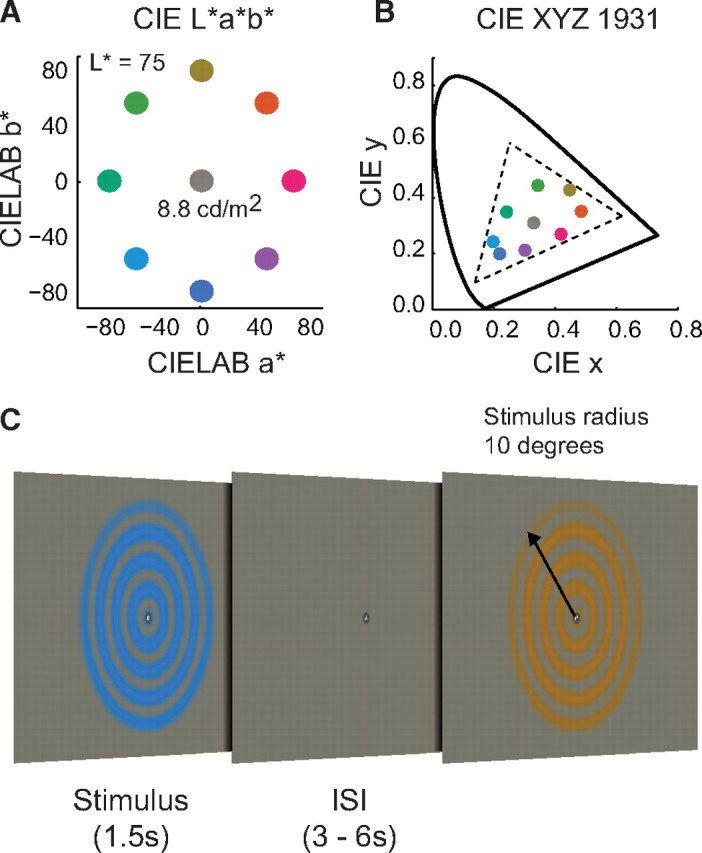
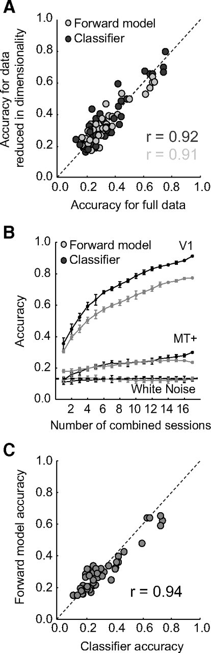
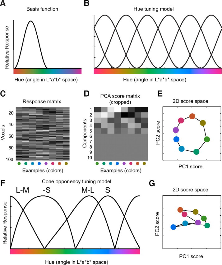
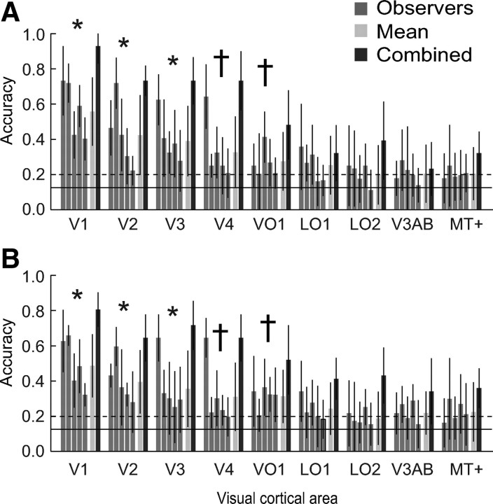
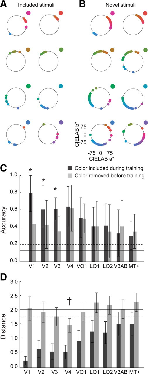
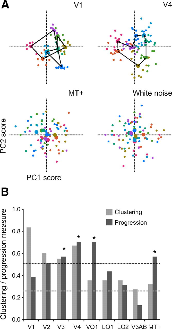
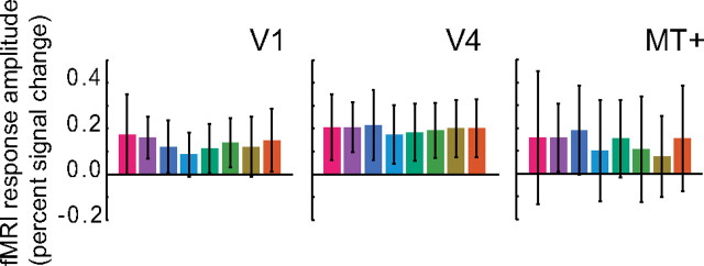
How is color represented by spatially distributed patterns of activity in visual cortex? Functional magnetic resonance imaging responses to several stimulus colors were analyzed with multivariate techniques: conventional pattern classification, a forward model of idealized color tuning, and principal component analysis (PCA). Stimulus color was accurately decoded from activity in V1, V2, V3, V4, and VO1 but not LO1, LO2, V3A/B, or MT+. The conventional classifier and forward model yielded similar accuracies, but the forward model (unlike the classifier) also reliably reconstructed novel stimulus colors not used to train (specify parameters of) the model. The mean responses, averaged across voxels in each visual area, were not reliably distinguishable for the different stimulus colors. Hence, each stimulus color was associated with a unique spatially distributed pattern of activity, presumably reflecting the color selectivity of cortical neurons. Using PCA, a color space was derived from the covariation, across voxels, in the responses to different colors. In V4 and VO1, the first two principal component scores (main source of variation) of the responses revealed a progression through perceptual color space, with perceptually similar colors evoking the most similar responses. This was not the case for any of the other visual cortical areas, including V1, although decoding was most accurate in V1. This dissociation implies a transformation from the color representation in V1 to reflect perceptual color space in V4 and VO1.

Figure 1.

Stimulus and experimental protocol. A, Location of the eight colors and gray point in CIE L*a*b* space. Colors were presented at a lightness of L* = 75 (8.8 cd/m²). B, The same eight colors and gray point in CIE 1931 xyz space. C, Stimuli were concentric sinusoidal gratings (spatial frequency, 0.5 cycles/°), within a circular aperture (10° radius), modulating from a center gray point to one of the eight locations in color space. Stimuli drifted either inward or outward, at a speed of 1°/s. Stimulus duration, 1.5 s. Interstimulus interval, 3–6 s in steps of 1.5 s.

Figure 2.

Comparison of methods. A, Comparison between decoding accuracies obtained with the full data (dimensionality = number of voxels) and accuracies obtained with the data after reducing it by means of PCA (dimensionality = number of components needed to explain 68% of the variance). Each point represents average decoding accuracy for one observer and ROI. Dark symbols, Maximum likelihood classifier. Light symbols, Forward model. Correlation coefficients (r values), Correlation in decoding accuracy between the full data and the reduced data for each decoder. B, Decoding accuracies obtained by combining data across sessions. Increasing the number of sessions dramatically increased V1 accuracies but only slightly increased MT+ accuracies. Replacing the data with white noise yielded chance performance. Error bars indicate SDs across runs (with 1 run at a time left out of training and used for testing accuracy). Dark curves and symbols, Maximum likelihood classifier. Light curves and symbols, Forward model classifier. C, Correlation between maximum likelihood classification and forward modeling classification accuracies. Each point corresponds to the mean decoding accuracy for one observer and ROI. Correlation coefficient (r value), Correlation in decoding accuracy between maximum likelihood classifier and forward model.

Figure 3.

Forward model. A, Idealized color tuning curve, modeled as a half-wave rectified and squared sinusoid. B, The response of a voxel was fitted with a weighted sum of six idealized color tuning curves, evenly spaced around the color circle, in CIE L*a*b* space. C, Simulated response amplitude matrix, for each voxel and each color. D, Matrix of principal component scores, computed by projecting the vector of response amplitudes (across voxels) onto each of the principal component vectors, ordered by the amount of variance they explain in the original response amplitudes. E, Plotting the first two principal component scores as coordinate pairs reconstructs the original color space. F, Cone-opponency model. LMS cone responses were calculated for the stimulus colors. Four cone-opponency channels (M–L, L–M, −S, and +S) were computed from the cone responses, half-wave rectified. G, The first two principal components of the simulated cone-opponency responses revealed results similar to those observed in V1.

Figure 4.

Color decoding. A, Decoding accuracies obtained with the maximum likelihood classifier, for each visual area. Gray bars, Decoding accuracies for individual observers. Light bars, Mean across observers. Dark bars, Accuracies obtained by combining the data across observers before classification. *p < 0.05, visual areas for which accuracies were significantly above chance in all observers (2-tailed permutation test); ^†p < 0.05, areas for which accuracies were significantly above chance in at least three of five observers. Error bars indicate SDs across runs (with 1 run at a time left out of training and used for testing accuracy). Solid line, Chance accuracy (0.125%). Dashed line, 97.5 percentile for chance accuracy, obtained by permutation tests (see Materials and Methods). The 97.5 percentiles were computed separately for each observer and visual area, but the average across observers/ROIs is shown here for simplicity. B, Decoding accuracies obtained using the forward model. Same format as in A.

Figure 5.

Reconstruction. A, Color reconstruction on the basis of V4 activity. Each point represents the color reconstructed for one run, using combined data from all sessions and observers, plotted in CIE L*a*b* space. The reconstructed colors from all sessions and observers cluster near the actual stimulus color, indicated in the top right of each panel. B, Reconstruction of novel colors, not included in training the forward model. Reconstructed colors again cluster near the actual stimulus color but with more spread than in A. C, Forward model decoding accuracies for included and novel colors. Error bars indicate SD of the accuracies over runs. *p < 0.05, visual areas for which there was a statistically significant difference when the test color was excluded from training (paired-sample t test). Solid line, Chance accuracy (0.125%). Dashed line, 97.5 percentile for chance accuracy, obtained by permutation tests (identical to Fig. 4). Areas V1, V2, and V3 show a significant decrease in decoding accuracy for novel colors, whereas areas V4 and VO1 show highly similar decoding accuracies for both included and novel colors. The accuracies for included colors in this figure are similar but not identical to the combined accuracies shown in Figure 4B. Each run is associated with one example per color. If we remove one color from training at a time and we leave one run out at a time, we can only predict one example per run (the example associated with the color excluded from training). The remaining colors in the run are not novel. Thus, for fair comparison, we determined the accuracy for included colors in the same way. D, Performance of the maximum likelihood classifier on included (black bars) and novel (gray bars) colors, quantified as the average distance between the color predicted by the maximum likelihood classifier and the novel color presented. Small distances indicate that the classifier predicted colors as perceptually similar, neighboring colors. The maximum distance was 4 (classifying a novel color as the opposite color on the hue circle), and the minimum distance in the case of included colors was 0 (correctly classifying a included color), or, in the case of novel colors, the minimum distance was 1 (classifying a novel color as its immediate neighbor). Error bars indicate SDs across runs (with 1 run at a time left out of training and used for testing accuracy). Solid line, Median distance as expected by chance. Dashed line, Statistical threshold (p < 0.05, two-tailed permutation test). ^†p < 0.05, visual areas for which the measured distance for novel colors was statistically smaller than expected by chance.

Figure 6.

Neural color spaces. A, Color spaces derived from the covariation, across voxels, in the responses to different stimulus colors, using data combined over all sessions and observers. In V4, the first two principal components (main source of variation) reveal a nearly circular progression (not self-intersecting) through color space, with similar colors evoking the most similar responses. This is not the case for V1 or MT+ activity, nor for white noise. Note, however, that V1 shows a more robust clustering of PCA scores, relative to the other areas. B, Clustering and progression of the color spaces derived from activity in each visual cortical area. Dashed lines, Chance levels for the progression (black) and clustering (gray) measures, computed by a permutation test (see Materials and Methods). All areas show clustering significantly higher than chance (p < 0.05, two-tailed permutation test). *p < 0.05, visual areas with a progression measure higher than chance (two-tailed permutation test). The relatively high progression score in MT+ is artifactual because the cluster centers were all near the origin of the space.

Figure 7.

Mean response amplitudes. Mean response amplitudes for each of the eight colors, averaged throughout each of three representative visual area ROIs, from a representative observer. In this observer, it is clear that the mean responses were not statistically different between colors. Similar results were found for other observers/ROIs. Error bars indicate SD of mean responses, averaged across voxels, over runs. See also Table 2.

References

1. Bartels A, Zeki S. The architecture of the colour centre in the human visual brain: new results and a review. Eur J Neurosci. 2000;12:172–193. - PubMed
1. Boynton GM, Engel SA, Glover GH, Heeger DJ. Linear systems analysis of functional magnetic resonance imaging in human V1. J Neurosci. 1996;16:4207–4221. - PMC - PubMed
1. Brainard DH. Cone contrast and opponent modulation color spaces. In: Kaiser P, Boynton RMB, editors. Human color vision. Washington, DC: Optical Society of America; 1996. pp. 563–579.
1. Brewer AA, Liu J, Wade AR, Wandell BA. Visual field maps and stimulus selectivity in human ventral occipital cortex. Nat Neurosci. 2005;8:1102–1109. - PubMed
1. Commission Internationale de l'Eclairage. Colorimetry. Ed 2. Vienna: Commission Internationale de l'Eclairage; 1986. CIE No. 152.
Publication types