Structure of deviations from optimality in biological systems

Abstract

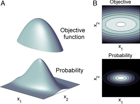
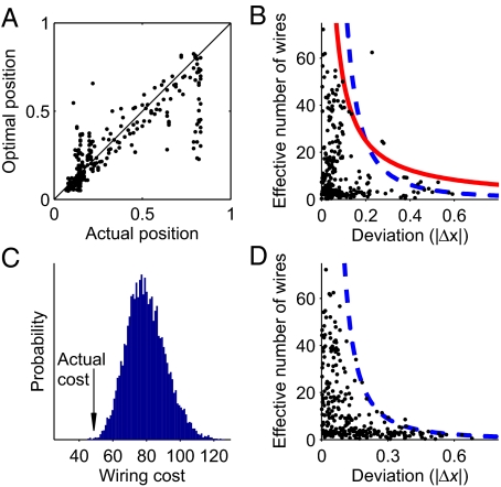
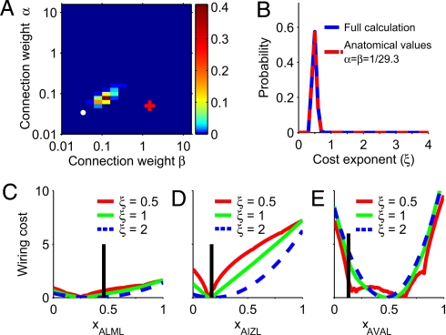
Optimization theory has been used to analyze evolutionary adaptation. This theory has explained many features of biological systems, from the genetic code to animal behavior. However, these systems show important deviations from optimality. Typically, these deviations are large in some particular components of the system, whereas others seem to be almost optimal. Deviations from optimality may be due to many factors in evolution, including stochastic effects and finite time, that may not allow the system to reach the ideal optimum. However, we still expect the system to have a higher probability of reaching a state with a higher value of the proposed indirect measure of fitness. In systems of many components, this implies that the largest deviations are expected in those components with less impact on the indirect measure of fitness. Here, we show that this simple probabilistic rule explains deviations from optimality in two very different biological systems. In Caenorhabditis elegans, this rule successfully explains the experimental deviations of the position of neurons from the configuration of minimal wiring cost. In Escherichia coli, the probabilistic rule correctly obtains the structure of the experimental deviations of metabolic fluxes from the configuration that maximizes biomass production. This approach is proposed to explain or predict more data than optimization theory while using no extra parameters. Thus, it can also be used to find and refine hypotheses about which constraints have shaped biological structures in evolution.

Fig. 1.

Suboptimal structure in a two-component model with objective Z(x₁,x₂) = x₁² + 5x₂². (A) (Upper) Parabolic objective function with slower decrease in the x₁ direction. (Lower) Probability resulting from Eq. 1, using as an example P(x→) = exp(−Z(x→)/0.4). The region of high probability extends further in the direction of x₁ because the objective decreases slower in this direction. (B) (Upper) Contour plots for the objective function (grayscale, lighter for higher values). (Lower) Contour plot for the probability (grayscale, lighter for higher values). Eq. 1 implies that isoprobability lines are the same than isoobjective lines.

Fig. 2.

Deviations of soma positions in C. elegans from the optimal positions of minimum wiring configuration. (A) Position of somas obtained by deterministic wiring cost minimization versus experimental values. Perfect match between deterministic optimization theory and experiment would fall on the diagonal. (B) Effective number of wires of each neuron (ω) versus experimental deviations from optimality (|Δx| ≡ |x_experimental−x_opt|). Larger deviations are expected for neurons with lower ω. Blue dashed line follows ω ∝ |Δx|⁻², and red solid line follows ω ∝ 1/|Δx|⁻¹. The three outliers (above the red line) are neurons DA6, AVAL, and AVAR. (C) Histogram of the wiring costs resulting from random redistribution of the deviations of somatic positions from their optima. Arrow indicates the cost of the actual configuration. Only 0.033% of the permutations have a lower cost. (D) Effective number of wires (ω) versus deviations obtained from a simulation performed by stochastic hill climbing with a Gaussian stochastic component added to wiring cost. Blue dashed line corresponds to the approximate theoretical prediction, ω ∝ |Δx|⁻².

Fig. 3.

Bayesian estimation of parameters in wiring cost function of C. elegans. (A) Probability of α (relative weight for neuron–neuron connections) and β (relative weight for neuron–muscle connections), according to the Bayesian estimator. Most probable values are α = 0.08, β = 0.13. These values are closer to the ones based on C. elegans anatomy, α = β = 1/29.3 (white dot), than to the ones fitting best the data by using deterministic wiring minimization, α = 0.05, β = 1.5 (red plus sign). (B) Probability for the cost exponent ξ. Most probable cost exponent is ξ = 0.49 ± 0.07. Results are identical using the complete Bayesian estimation taking into account all values of α, β (blue) as when fixing α, β to their anatomically based values, α = β = 1/29.3 (red). (C–E) Wiring cost along the direction of the position of neurons ALML, AIZL, and AVAL with all other neurons fixed in their experimental positions, for wiring cost exponents ξ = 0.5 (red), ξ = 1.0 (green), and ξ = 2.0 (blue). Black vertical bars: actual soma position. AVAL is far from its optimal position but sits close to a local minimum. The same happens for AVAR (data not shown). DA6 does not improve significantly with the new parameters.

Fig. 4.

Deviations from optimality in the metabolic network of E. coli. (A) Optimal fluxes for maximization of biomass production versus experimental fluxes. Perfect correspondence of deterministic optimization and data would fall in the diagonal. Bars give experimental error reported in ref. . (B) Optimal fluxes for maximization of ATP production versus experimental fluxes. (C) Theoretical and experimental deviations from the optimum for biomass production as objective. For each flux, colors show the value of the objective function (relative to the optimum) as a function of the deviation of the flux. Dark red is reserved for a value of objective of exactly 1, so that maxima are clearly seen. Eq. 1 implies that the fluxes should be at the red regions. White dots are located at the experimental deviations. (D) Same as C for ATP production as objective. (E) P value from significance analysis for all possible values of Δ. Red line: significance of the theoretical results using biomass production as objective. Blue line: using ATP production as objective. Black dashed line: P = 0.05 significance line.

References

1. Barton NH, Briggs DEG, Eisen JA, Goldstein DB, Patel NH. Evolution. Cold Spring Harbor, NY: Cold Spring Harbor Lab Press; 2007.
1. Alexander RM. Optima for Animals. Princeton: Princeton Univ Press; 1996.
1. Parker GA, Maynard Smith J. Optimality theory in evolutionary biology. Nature. 1990;348:27–33.
1. Freeland SJ, Hurst LD. The genetic code is one in a million. J Mol Evol. 1998;47:238–248. - PubMed
1. Itzkovitz S, Alon U. The genetic code is nearly optimal for allowing additional information within protein-coding sequences. Genome Res. 2007;17:405–412. - PMC - PubMed
Publication types