Intervening inhibition underlies simple-cell receptive field structure in visual cortex

Abstract

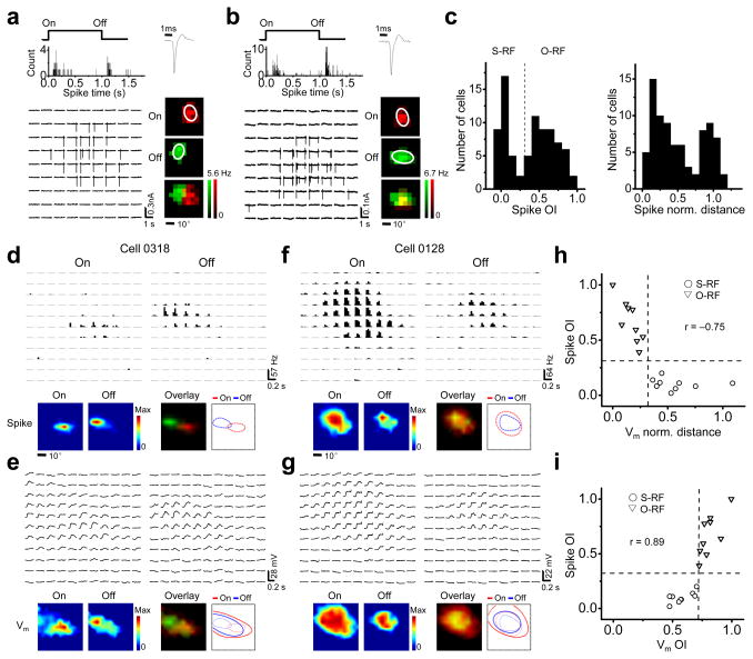
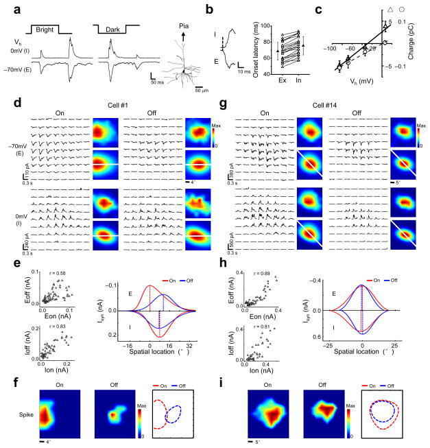
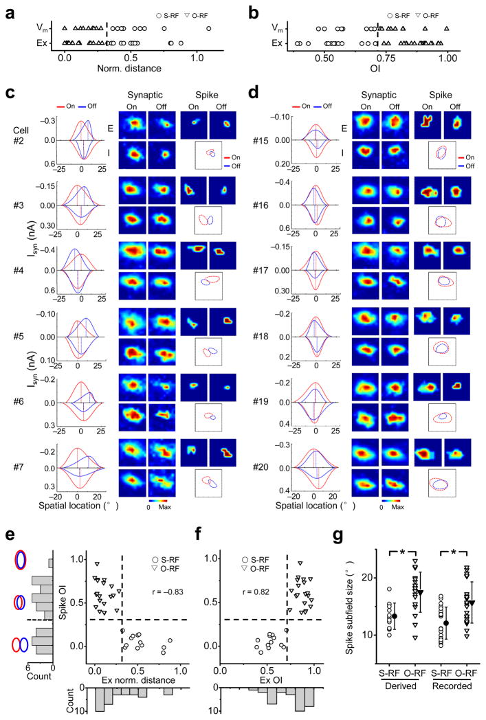
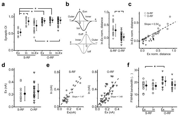
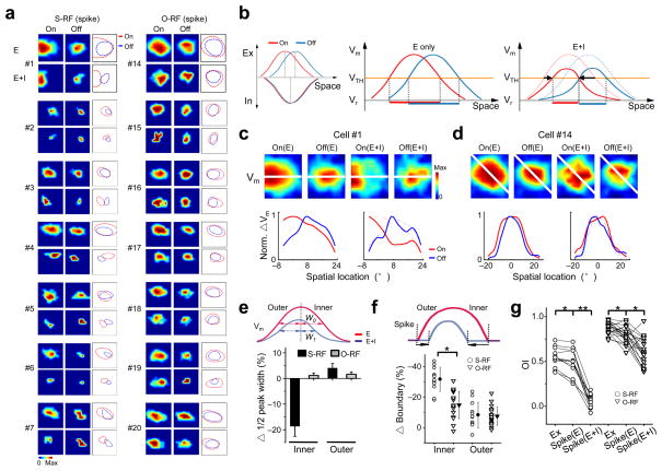
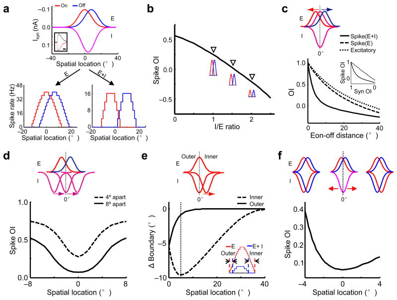
Synaptic inputs underlying spike receptive fields are important for understanding mechanisms of neuronal processing. Using whole-cell voltage-clamp recordings from neurons in mouse primary visual cortex, we examined the spatial patterns of their excitatory and inhibitory synaptic inputs evoked by On and Off stimuli. Neurons with either segregated or overlapped On/Off spike subfields had substantial overlaps between all the four synaptic subfields. The segregated receptive-field structures were generated by the integration of excitation and inhibition with a stereotypic 'overlap-but-mismatched' pattern: the peaks of excitatory On/Off subfields were separated and flanked colocalized peaks of inhibitory On/Off subfields. The small mismatch of excitation/inhibition led to an asymmetric inhibitory shaping of On/Off spatial tunings, resulting in a great enhancement of their distinctiveness. Thus, slightly separated On/Off excitation, together with intervening inhibition, can create simple-cell receptive-field structure and the dichotomy of receptive-field structures may arise from a fine-tuning of the spatial arrangement of synaptic inputs.

Figure 1

Membrane potential (V_m) responses underlying S-RF and O-RF structures in layer 2/3 of the mouse V1. (a–b) Example S-RF (a) and O-RF (b) cells. Top left, the peri-stimulus-spike-time histograms (PSTH) for evoked spikes. “On” and “Off” mark the onset and offset of the stimuli respectively. Top right, the spike shape. Bottom left, each small trace represents the recorded spike response (vertical deflections) in one trial to a unit stimulus displayed at the corresponding spatial location. Bottom right, color maps of the spike subfields. The white ellipses depict the outlines of the spike subfields determined by Gaussian fittings. (c) Left, histogram of OI of spike subfields (spike OI) for the recorded excitatory neurons. The dash line marks OI = 0.33. Right, histogram of normalized distance between the peaks of spike On and Off subfields. (d) Spike RF for an example S-RF cell. Top, each small trace represents the PSTH for spike responses to a unit On or Off stimulus. Bottom, color maps and outlines of spike On/Off subfields. Color scale: 14.8 (On) and 39.1 Hz (Off). (e) V_m responses of the same cell in d. Top, traces of average V_m responses. Bottom, color maps and outlines of V_m subfields. Color scale: 22 (On) and 26 mV (Off). (f–g) An example O-RF cell. Data are presented in the same way as in d–e. Color scale: 42.3 and 21.5 Hz in f; 20 and 18 mV in g. (h) Spike OI versus normalized distance between the peaks of V_m subfields. The two dash lines (OI = 0.33, norm. distance = 0.32) separate S-RF and O-RF structures. “r”, correlation coefficient. (i) Spike OI versus OI of V_m subfields (V_m OI). The vertical and horizontal lines mark V_m OI = 0.71 and spike OI = 0.33 respectively.

Figure 2

Synaptic subfields examined by voltage-clamp recordings. (a) Individual synaptic responses of a layer 2/3 pyramidal neuron to stimuli displayed at the same location. Scale: 118 (E) and 203 pA (I). Right, the reconstructed morphology of the cell. (b) Left, onset phase of synaptic responses. The onset of the excitatory response was marked by dash line. Scale: 80 (E) and 160 pA (I). Right, onset latencies of excitatory (Ex) and inhibitory (In) synaptic responses. The values from the same cell are connected with a line. Solid symbol = mean, error bar = SD. (c) I–V curves for a cell under white noise stimulation. Synaptic charges were measured in a 0–5ms (circle) and 10–150ms (triangle) time window after the onset of excitatory synaptic responses. (d–f) A putative S-RF cell. (d) Arrays of trial-averaged excitatory (E) and inhibitory (I) synaptic responses to On and Off stimuli. Color maps are the smoothed (top) and skew-normal fitted (bottom) synaptic subfields. White lines pass through the peaks of the excitatory On and Off subfields. Color scale: 109, 73, 236, and 178 pA for Eon, Eoff, Ion and Ioff respectively. (e) Left, correlation between the strengths of synaptic responses (Eon-Eoff, Ion-Ioff). Right, spatial tuning curves of the four synaptic inputs along the white lines in d. Dash lines mark their peaks. (f) Derived spike subfields of the same cell and their boundaries. Color scale: 25 (On) and 10 Hz (Off). (g–i) Synaptic subfields of a putative O-RF cell. Data are presented in the same manner as in d–f. Color scale in g: 381, 352, 560 and 412 pA (Eon, Eoff, Ion, Ioff). Color scale in i: 25 (On) and15 Hz (Off).

Figure 3

Grouping of cells based on the structure of synaptic subfields. (a) The distributions of the normalized distances between the peaks of V_m On/Off subfields, and between the excitatory On/Off subfields (Ex). The two distributions are not different (Mann-Whitney test, p = 0.14). The dash line marks norm. distance = 0.32, which was used to group the cells from V-clamp recordings. (b) The distributions of the OIs of V_m and excitatory subfields. Mann-Whitney test, p = 0.21. The dash line marks OI = 0.71, which separated the cells from V-clamp recordings the same as in a. (c) Synaptic subfields and derived spike subfields of six putative S-RF cells. For each cell, shown from left to right are the synaptic tuning curves in the slice that passes through the peaks of the Eon and Eoff, the four synaptic subfields, the derived spike subfields and the superimposed outlines of fitted spike subfields. Color scale: 337, 404,543, 528 pA for synaptic subfields (in the sequence of Eon, Eoff, Ion, Ioff), 15, 10 Hz for spike On/Off subfields in cell #2; 163, 165, 288, 196 pA, 10, 15 Hz in cell #3; 280, 342, 638, 854 pA, 10, 10 Hz in cell #4; 122, 106, 142, 141 pA, 10, 10 Hz in cell #5; 225, 153, 245, 161 pA, 15, 20 Hz in cell #6; 311, 184, 412, 149 pA, 10, 5 Hz in cell #7. (d) Six putative O-RF cells. Plots are organized in the same way as in c. Color scale: 74, 54, 141, 82 pA, 5, 10 Hz in cell #15; 398, 347, 595, 563 pA, 10, 10 Hz in cell #16; 141, 154, 298, 145 pA, 15, 15 Hz in cell #17; 187, 172, 218, 173 pA, 15, 15 Hz in cell #18; 232, 154, 356, 329 pA, 20, 5 Hz in cell #19; 280, 253, 415, 221 pA, 15, 15 Hz in cell #20. (e) OI of derived spike subfields versus the normalized distance between the peaks of the Eon and Eoff for all recorded neurons (n = 33). The vertical and horizontal dash lines mark Ex norm. distance = 0.32 and spike OI = 0.33 respectively. Left, histogram of spike OI. The schematic drawings depict the extent of overlap between two identical subfields for OI = 0, 0.5 and 1 respectively. Bottom, histogram of Ex norm. distance. (f) OI of derived spike subfields vs. the OI between the Eon and Eoff. The vertical and horizontal dash lines mark Ex OI = 0.71 and spike OI = 0.33 respectively. Bottom, the histogram of Ex OI. (g) The distribution of the subfield size of the derived and recorded spike responses. Solid symbol = mean, error bar = SD. *, p < 0.01, t-test.

Figure 4

Summary of the spatial relationships between synaptic subfields. (a) The distributions of OIs between the Eon and Eoff (Ex), the Ion and Ioff (In) as well as between the excitatory and inhibitory subfields of the same contrast (In-Ex). Solid symbol = mean, error bar = SD. *, p < 1e–5, t-test. (b) Left, we defined the inner side of an excitatory tuning curve as the one facing towards the other excitatory tuning curve of the opposite contrast. The value of In-Ex distance is positive if the peak of the inhibitory field is located on the inner side of the excitatory field of the same contrast, but negative if it is on the outer side. Right, the distribution of the normalized In-Ex distance. Solid symbol = mean, error bar = SD. *, p < 1e–6, t-test, n = 26 (S-RF) and 40 (O-RF). (c) Normalized In-Ex distance (averaged for On and Off subfields) versus the normalized distance between the peaks of the Eon and Eoff. The dash line is the best-fit linear regression line. Arrow points the only cell that would be grouped differentlyunder TwoStep Cluster analysis. (d) The maximal amplitude of the excitatory currents. Solid symbol = mean, error bar = SD. P = 0.34, t-test. (e) The maximum strength of inhibitory input (In) versus that of excitatory input (Ex) in the same subfield. The dash line shows the best-fit linear regression line. (f) The full-width at half-maximum bandwidth of excitatory and inhibitory spatial tuning curves. Solid symbol = mean, error bar = SD. *, p = 0.02, t-test.

Figure 5

The inhibitory mechanism for the generation of the S-RF structure. (a) Derived spike subfields without (E) and with the integration of inhibition (E+I) of the cells in Figure 2 and 3. Dashed curves represent the outlines of the subfields. Color scale in the order of On(E), Off(E), On(E+I) and Off(E+I): from cell #1 to #7, 30, 25, 25, 10 Hz; 20, 15, 15, 10 Hz; 25, 20, 10, 15 Hz; 25, 20, 10, 10 Hz; 15, 10, 10, 10 Hz; 25, 20, 15, 20 Hz; 15, 10, 10, 5 Hz; and from cell #14 to #20: 35, 20, 25, 15 Hz; 20, 15, 5, 10 Hz; 30, 15, 10, 10 Hz; 25, 20, 15, 15 Hz; 20, 15, 15, 15 Hz; 30, 20, 20, 5 Hz; 20, 15, 15, 15 Hz. (b) Schematic drawings to show how inhibition plays a role in the generation of S-RFs. Left, the spatial tuning curves of excitatory and inhibitory inputs. The peak locations are marked by dotted lines. Middle, the spatial tuning curves of V_m responses without inhibition. V_TH and V_r stand for spike threshold and resting potential respectively. The thick red and blue lines below the tuning curves represent the one dimensional regions of the suprathreshold On/Off responses respectively. Note that they overlap significantly. Right, the V_m tuning curves after integrating inhibition (solid curves), overlayed with the tuning curves without inhibition (dashed). The suprathreshold On/Off response regions are now segregated. Arrows indicate the shrinkage of suprathreshold subfield boundaries. (c) Top, color maps of V_m responses derived without (E) and with (E+I) integrating inhibition for cell #1. Scale from left to right: 47, 40, 39, 26 mV. White line was defined the same as before. Bottom, normalized spatial tuning curves of V_m responses along the white line, in the absence (left) and presence (right, solid) of inhibition. Note a strong suppression of the right part of the On tuning curve. (d) Similar plottings for cell #14. Scales: 54, 53, 32, 36 mV. (e) The percentage change in the half-peak width of the V_m tuning curve after integrating inhibition. Top, schematic drawings of V_m tuning curves before and after integrating inhibition, with the half-peak widths at the inner side labelled by W₀ and W₁ respectively. The percentage change is then defined as (W₁ − W₀)/W, where W is the full-width at half-maximum of the tuning curve without inhibition. Error bar = SE. (f) Percentage shift of spike subfield boundaries after integrating inhibition. Arrows in the schematic drawings depict the boundary shift on the inner and outer side. The absolute value was divided by the size of spike subfields without inhibition to obtain the percentage shift. (g) OIs between Eon and Eoff (Ex), and between spike On/Off subfields derived without (spike(E)) and with inhibition (spike(E+I)). Values for the same cell are connected with lines. *, p < 0.005; **, p < 0.0001, paired t-test.

Figure 6

Modelling how the spatial relationships between synaptic subfields affect the segregation of spike On/Off subfields. (a) Top, the spatial tuning curves of synaptic currents (I_syn) used in the model. Inset, the temporal profiles of evoked excitatory (red) and inhibitory currents (black). Scale: 125 ms. Bottom, the tuning curves of spike responses without (left) and with inhibition (right). (b) With the strength of excitation fixed at 0.1nA, the spike OI decreases as the level of inhibition increases. Inset, spike tuning curves at I/E ratio=1, 1.5, 2. (c) Top, modelling scenario: the excitatory On (red) and Off (blue) subfields are initially co-localized with the overlapping inhibitory fields (purple) and then move away from each other at the same speed. Bottom, OIs between the Eon and Eoff (dotted), and between spike subfields without (dashed) and with inhibition (solid) versus the distance between the peaks of the Eon and Eoff. Inset, spike OI versus the OI between the Eon and Eoff (Syn OI). (d) Top, the peaks of the Eon and Eoff are separated by 4° (dashed) or 8° (solid), and the overlapping inhibitory subfields move together across different locations. Bottom, spike OI versus the spatial location of the inhibitory fields. (e) Top, the Ion is initially co-localized with the Eon and then moves in the direction towards the Eoff (not shown). Bottom, shift of the spike subfield boundary after integrating inhibition versus the location of the Ion peak. The dotted line marks the location of inhibitory subfield (~5°) where it shrinks the inner boundary most. Inset, spike tuning curves without (red) and with inhibition (blue) when the Ion peak is located at 4°. Arrows mark the boundary shifts on the two sides. (f) Top, the positions of the excitatory subfields are fixed, with an 8° separation. The initially overlapping inhibitory subfields move in opposite directions to form either exquisitely balanced excitation and inhibition (left) or an antagonistic configuration similar to the push-pull (right). Bottom, spike OI versus the location of the Ion peak, which equals to −4°, 0° and 4° for the three above scenarios respectively.

References

1. Hubel DH, Wiesel TN. Receptive fields, binocular interaction and functional architecture in the cat’s visual cortex. J Physiol. 1962;160:106–154. - PMC - PubMed
1. Heggelund P. Quantitative studies of the discharge fields of single cells in cat striate cortex. J Physiol. 1986;373:277–292. - PMC - PubMed
1. Hirsch JA, Alonso JM, Reid RC, Martinez LM. Synaptic integration in striate cortical simple cells. J Neurosci. 1998;18:9517–9528. - PMC - PubMed
1. Troyer TW, Krukowski AE, Priebe NJ, Miller KD. Contrast-invariant orientation tuning in cat visual cortex: feedforward tuning and correlation-based intracortical connectivity. J Neurosci. 1998;18:5908–5927. - PMC - PubMed
1. Miller KD. Understanding layer 4 of the cortical circuit: a model based on cat V1. Cereb Cortex. 2003;13:73–82. - PubMed
Publication types