

Distributed lag and spline modeling for predicting energy expenditure from accelerometry in youth
- PMID: 19959770
- PMCID: PMC2822669
- DOI: 10.1152/japplphysiol.00374.2009
Distributed lag and spline modeling for predicting energy expenditure from accelerometry in youth
Abstract
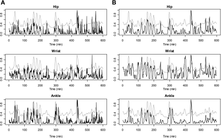
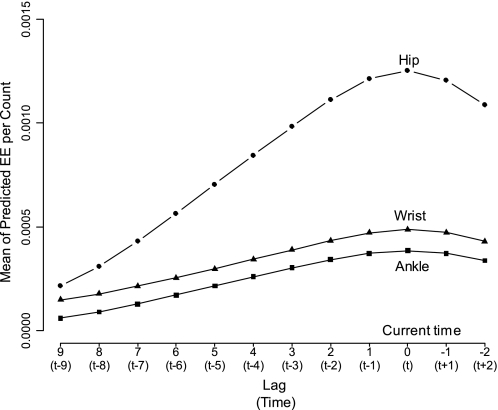
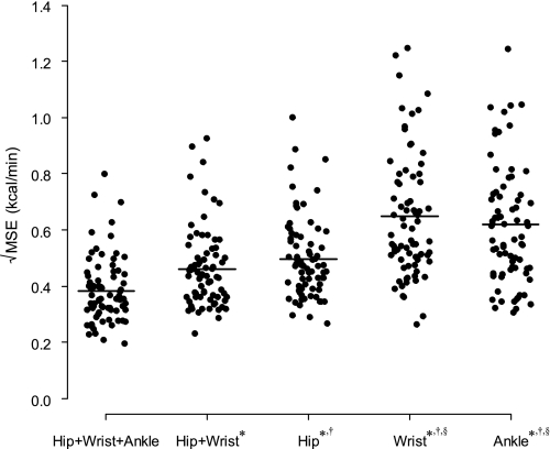
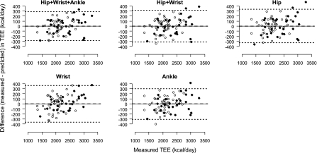
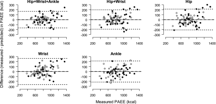
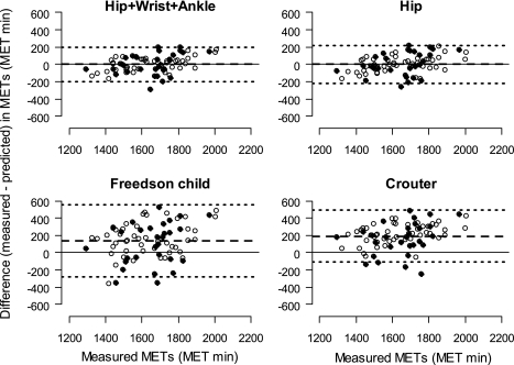
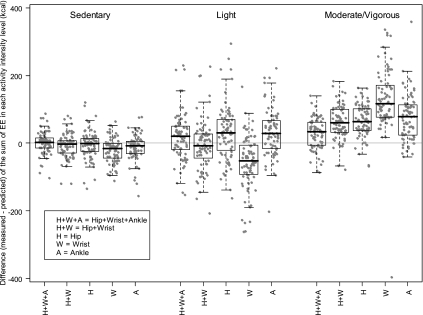
Movement sensing using accelerometers is commonly used for the measurement of physical activity (PA) and estimating energy expenditure (EE) under free-living conditions. The major limitation of this approach is lack of accuracy and precision in estimating EE, especially in low-intensity activities. Thus the objective of this study was to investigate benefits of a distributed lag spline (DLS) modeling approach for the prediction of total daily EE (TEE) and EE in sedentary (1.0-1.5 metabolic equivalents; MET), light (1.5-3.0 MET), and moderate/vigorous (> or = 3.0 MET) intensity activities in 10- to 17-year-old youth (n = 76). We also explored feasibility of the DLS modeling approach to predict physical activity EE (PAEE) and METs. Movement was measured by Actigraph accelerometers placed on the hip, wrist, and ankle. With whole-room indirect calorimeter as the reference standard, prediction models (Hip, Wrist, Ankle, Hip+Wrist, Hip+Wrist+Ankle) for TEE, PAEE, and MET were developed and validated using the fivefold cross-validation method. The TEE predictions by these DLS models were not significantly different from the room calorimeter measurements (all P > 0.05). The Hip+Wrist+Ankle predicted TEE better than other models and reduced prediction errors in moderate/vigorous PA for TEE, MET, and PAEE (all P < 0.001). The Hip+Wrist reduced prediction errors for the PAEE and MET at sedentary PA (P = 0.020 and 0.021) compared with the Hip. Models that included Wrist correctly classified time spent at light PA better than other models. The means and standard deviations of the prediction errors for the Hip+Wrist+Ankle and Hip were 0.4 +/- 144.0 and 1.5 +/- 164.7 kcal for the TEE, 0.0 +/- 84.2 and 1.3 +/- 104.7 kcal for the PAEE, and -1.1 +/- 97.6 and -0.1 +/- 108.6 MET min for the MET models. We conclude that the DLS approach for accelerometer data improves detailed EE prediction in youth.
Figures
Similar articles
-
Validation of the ActiGraph two-regression model for predicting energy expenditure.Med Sci Sports Exerc. 2010 Sep;42(9):1785-92. doi: 10.1249/MSS.0b013e3181d5a984. Med Sci Sports Exerc. 2010. PMID: 20142778 Free PMC article.
-
A random forest classifier for the prediction of energy expenditure and type of physical activity from wrist and hip accelerometers.Physiol Meas. 2014 Nov;35(11):2191-203. doi: 10.1088/0967-3334/35/11/2191. Epub 2014 Oct 23. Physiol Meas. 2014. PMID: 25340969 Free PMC article.
-
Prior automatic posture and activity identification improves physical activity energy expenditure prediction from hip-worn triaxial accelerometry.J Appl Physiol (1985). 2018 Mar 1;124(3):780-790. doi: 10.1152/japplphysiol.00556.2017. Epub 2017 Nov 30. J Appl Physiol (1985). 2018. PMID: 29191980
-
Usefulness of motion sensors to estimate energy expenditure in children and adults: a narrative review of studies using DLW.Eur J Clin Nutr. 2017 Mar;71(3):331-339. doi: 10.1038/ejcn.2017.2. Epub 2017 Feb 1. Eur J Clin Nutr. 2017. PMID: 28145419 Review.
-
Statistical considerations in the analysis of accelerometry-based activity monitor data.Med Sci Sports Exerc. 2012 Jan;44(1 Suppl 1):S61-7. doi: 10.1249/MSS.0b013e3182399e0f. Med Sci Sports Exerc. 2012. PMID: 22157776 Review.
Cited by
-
Separating bedtime rest from activity using waist or wrist-worn accelerometers in youth.PLoS One. 2014 Apr 11;9(4):e92512. doi: 10.1371/journal.pone.0092512. eCollection 2014. PLoS One. 2014. PMID: 24727999 Free PMC article.
-
Ankle Accelerometry for Assessing Physical Activity Among Adolescent Girls: Threshold Determination, Validity, Reliability, and Feasibility.Res Q Exerc Sport. 2015;86(4):397-405. doi: 10.1080/02701367.2015.1063574. Epub 2015 Aug 19. Res Q Exerc Sport. 2015. PMID: 26288333 Free PMC article.
-
Estimation of daily energy expenditure in pregnant and non-pregnant women using a wrist-worn tri-axial accelerometer.PLoS One. 2011;6(7):e22922. doi: 10.1371/journal.pone.0022922. Epub 2011 Jul 29. PLoS One. 2011. PMID: 21829556 Free PMC article.
-
Validation of the ActiGraph two-regression model for predicting energy expenditure.Med Sci Sports Exerc. 2010 Sep;42(9):1785-92. doi: 10.1249/MSS.0b013e3181d5a984. Med Sci Sports Exerc. 2010. PMID: 20142778 Free PMC article.
-
Toddler physical activity study: laboratory and community studies to evaluate accelerometer validity and correlates.BMC Public Health. 2016 Sep 6;16(1):936. doi: 10.1186/s12889-016-3569-9. BMC Public Health. 2016. PMID: 27600404 Free PMC article.
References
-
- Actigraph Actigraph GT1M Monitor/ ActiTrainer and ActiLife Lifestyle Monitor Software User Manuel. Pensacola, FL: Actigraph, LLC, 2007
-
- Bland JM, Altman DG. Statistical methods for assessing agreement between two methods of clinical measurement. Lancet 1: 307–310, 1986 - PubMed
-
- Chen KY, Bassett DR., Jr The technology of accelerometry-based activity monitors: current and future. Med Sci Sports Exercise 37: S490–500, 2005 - PubMed
-
- Cleveland WS. Robust locally weighted regression and smoothing scatterplots. J Am Stat Assoc 74: 829–836, 1979
Publication types
MeSH terms
Grants and funding
LinkOut - more resources
Full Text Sources
Medical
Miscellaneous