Collective dynamics in human and monkey sensorimotor cortex: predicting single neuron spikes

Abstract

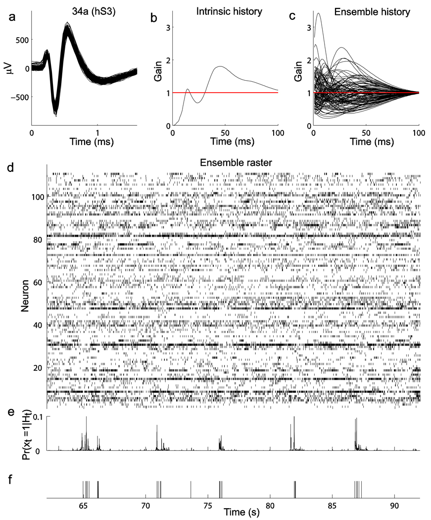
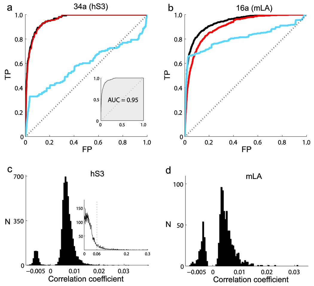
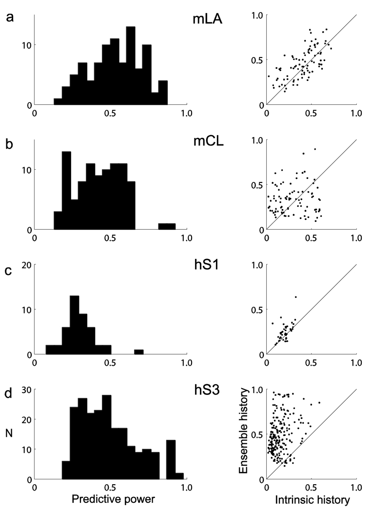
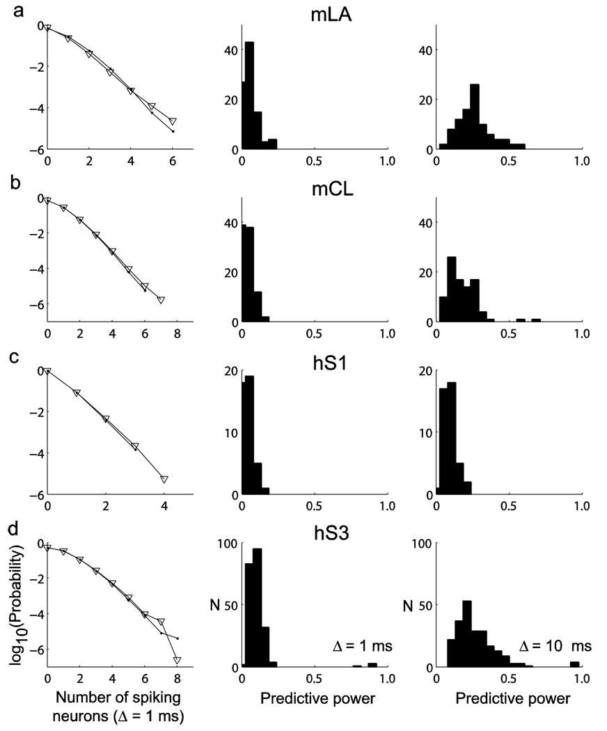
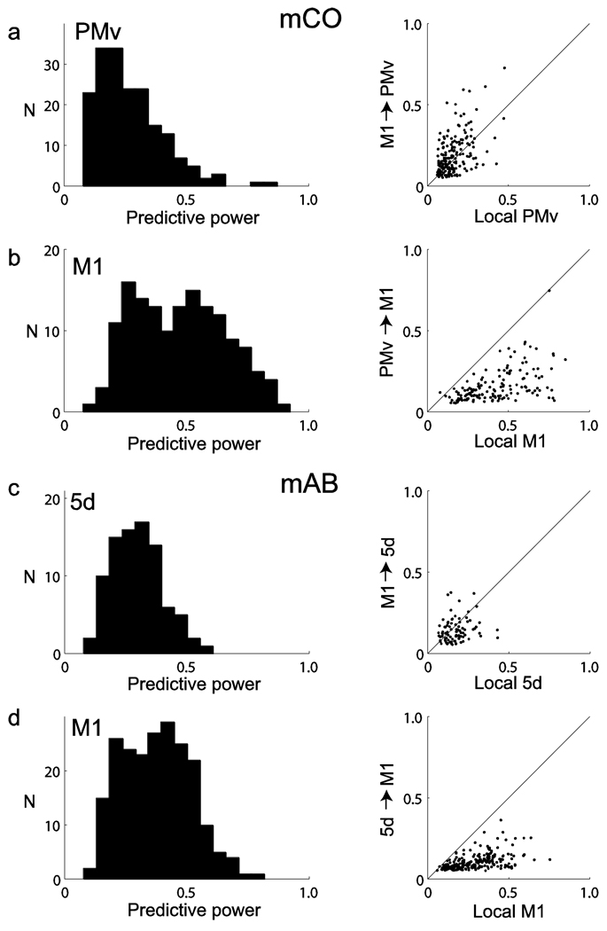
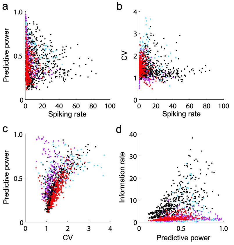
Coordinated spiking activity in neuronal ensembles, in local networks and across multiple cortical areas, is thought to provide the neural basis for cognition and adaptive behavior. Examining such collective dynamics at the level of single neuron spikes has remained, however, a considerable challenge. We found that the spiking history of small and randomly sampled ensembles (approximately 20-200 neurons) could predict subsequent single neuron spiking with substantial accuracy in the sensorimotor cortex of humans and nonhuman behaving primates. Furthermore, spiking was better predicted by the ensemble's history than by the ensemble's instantaneous state (Ising models), emphasizing the role of temporal dynamics leading to spiking. Notably, spiking could be predicted not only by local ensemble spiking histories, but also by spiking histories in different cortical areas. These strong collective dynamics may provide a basis for understanding cognition and adaptive behavior at the level of coordinated spiking in cortical networks.

Figure 1

History point process models, intrinsic and ensemble history effects, and conditional spiking probabilities. Neuron 34a (hS3, session 2) was chosen as the example target neuron. (a) Waveforms corresponding to all sorted spikes for neuron 34a used in these analyses are shown. (b) Intrinsic spiking history. The curve represents the estimated temporal filter for the intrinsic history. Values below or above 1 correspond to a decrease or increase, respectively, in spiking probability contributed by a spike at a previous time specified in the horizontal coordinate. Refractory and recovery period effects after a spike, followed by an increase in spiking probability at longer time lags (40–100 ms), can be seen. This late intrinsic history effect might also reflect network dynamics. (c) Ensemble spiking history effects. Each curve represents the temporal filter corresponding to a particular input neuron to cell 34a. Many input neurons contributed biphasic effects: for example, an increase in spiking probability followed by a decrease, or vice-versa. All of the examined target neurons in our datasets showed qualitatively similar temporal filters. (d) Spike raster for all of the 110 neurons recorded in hS3 over a short, continuous time period. (e) Predicted spiking probabilities for the target neuron 34a were computed from the estimated intrinsic and ensemble temporal filters and the spike trains shown in b, c and d, respectively. (f) Observed spike train for neuron 34a in the same period.

Figure 2

Prediction of single-neuron spiking and weak pair-wise correlations. (a) ROC curves for neuron 34a (human participant hS3, n = 110 neurons, session 2, 240,000 samples). FP and TP denote false- and true-positive prediction rates, respectively. The diagonal line corresponds to the expected chance prediction. The black, red and blue ROC curves correspond to the prediction based on full history models, only the ensemble histories, or only the neuron’s own spiking history, respectively. The inset shows the AUC corresponding to the ROC curve for the ensemble history model. (b) ROC curves for neuron 16a (monkey mLA, n = 45, session 2, 1,230,857 samples). 95% confidence intervals for the AUC chance level resulted in 0.51 ± 0.004 and 0.51 ± 0.017 for target neurons 16a and 34a, respectively. These narrow confidence intervals (data not shown) were typical for the recorded neurons. (c) Distribution of Pearson correlation coefficients computed over all of the neuron pairs for hS3 (1-ms time bins). N corresponds to the number of neuron pairs. Each of these correlation coefficients corresponds to the extremum value of the cross-correlation function computed for time lags in the interval ± 500 ms. Inset, normalized absolute (extremum) correlation coefficients for all of the neuronal pairs in the ensemble from hS3 computed for spike counts in 50-ms time bins; about 90% of the pairs had a correlation value smaller than 0.06 (vertical line). (d) Distribution of correlation coefficients computed over all of the neuron pairs for mLA (1-ms time bins).

Figure 3

Predictive power of intra-areal (M1) ensemble histories. (a–d) Prediction was substantial, as shown by the distributions of predictive power corresponding to target neurons from subjects mLA (a), mCL (b), hS1 (c) and hS3 (d). Each distribution includes target neurons recorded in two different sessions (mLA: n = 45, n = 45; mCL: n = 47, n = 44; hS1: n = 22, n = 21; hS3: n = 108, n = 110). The left column shows the distribution of predictive power based on the full history model and the right column compares the predictive power of the two (intrinsic and ensemble) history components separately. The predictive power measure is based on the AUC scaled and corrected for chance level prediction. It ranges from 0 (no predictive power) to 1 (perfect prediction). For many neurons, the predictive power of separate components (intrinsic and ensemble) could add to a value larger than 1 or result in a larger predictive power than that obtained by the full history model. This indicates that there was some redundancy in the information conveyed by these two components. The numbers of predicted samples (1-ms time bins) were 864,657 and 1,230,857 for mLA, 1,220,921 and 1,361,811 for mCL, 240,000 in both sessions for hS1 and 240,000 in both sessions for hS3.

Figure 4

Predictive power of instantaneous collective states (Ising models). (a–d) The distributions of instantaneous collective states were approximated via maximum entropy distributions constrained on empirical mean spiking rates and zero time-lag pair-wise correlations. The left column shows the empirical distribution of the observed number of multi-neuron spike coincidences in the ensemble (Δ = 1 ms) and the distribution generated from the maximum entropy model via Gibbs sampling (∇). The middle column shows the distribution of predictive power values. Predictive power was computed for each target neuron separately, with the instantaneous or simultaneous collective state defined at a temporal resolution of 1 ms. For each given neuron, predictions were determined by a conditional spiking probability derived from the maximum entropy joint distribution model and knowledge of all of the (n – 1) neurons’ simultaneous states. The right column shows the distribution of predictive power when the instantaneous state was defined at a coarser temporal resolution of 10 ms. In that case, time bins containing more than one spike were set to 1. For each monkey and human participant, data from two sessions were used in these analyses. The rows correspond to mLA (n = 45, n = 45, a), mCL (n = 47, n = 44, b), hS1 (n = 22, n = 21, c) and hS3 (n = 108, n = 110, d).

Figure 5

Predictive power of intra- and inter-areal neuronal ensemble histories. Predictive power of inter-areal ensemble history was also substantial. (a) Left, distribution of predictive power values for target neurons in area PMv (subject mCO), which were recorded during free reach-grasp movements. Predictive power was computed from full history models that also included spiking histories in M1. Right, comparison of the power of intra (PMv, n = 77, n = 109) and inter-areal (M1, n = 148, n = 109) ensemble histories to predict spiking in PMv. The predictive power M1→PMv tended to be higher than the local PMv→PMv in this case, where the number of neurons recorded in M1 was larger than in PMv. In contrast, additional analyses using balanced-size ensembles indicated that intra-areal predictive power was actually slightly higher (Supplementary Fig. 5). (b) Left, distribution of predictive power for target neurons in M1. Predictive power was computed from full history models that also included spiking histories in PMv. Right, comparison of the power of the intra (M1) and inter-areal (PMv) ensemble histories to predict spiking in M1. (c,d) Data are presented as in a and b, but were computed for parietal 5d (n = 41, n = 47) and M1 (n = 104, n = 110), recorded from monkey mAB during a planar pursuit tracking task. The numbers of predicted samples were 212,028 and 99,008 for mCO (sessions 1 and 2, respectively) and 416,162 and 472,484 for mAB (sessions 1 and 2, respectively).

Figure 6

Predictive power, mean spiking rates, spike train irregularity and information rates. Each dot corresponds to one of the 1,187 target neurons recorded from two human participants and four monkeys, three different cortical areas and four different tasks. Each color relates to one of the different tasks. (a) The predictive power of full history models versus the mean spiking rate (in spikes per s) of the target neurons is shown. (b) Coefficient of variation (CV) of the inter-spike time intervals versus spiking rates. (c) Predictive power of full history models versus coefficients of variation of the predicted spiking activity. Lower coefficients indicate more regular spike trains. Coefficients around 1 and below tended to correspond to a broad range of predictive power, whereas higher coefficients tended to cluster around intermediate predictive power values. In summary, the predictive power of history models did not seem to depend, in a simple manner, on mean spiking rates or on the level of irregularity of the spiking activity. (d) Predictive power versus the information rate (in bits per s) involved in the prediction. Approximately equal predictive power could relate to a broad range of information rates. Blue: point-to-point reaching, monkeys mLA and mCL, area M1; purple: neural cursor control, participants hS1 and hS3, area M1; black: free reach and grasp task, monkey mCO, areas M1 and PMv; red: pursuit tracking task, monkey mAB, areas M1 and 5d.

References

1. Braitenberg V, Schüz A. Cortex: Statistics and Geometry of Neuronal Connectivity. New York: Springer-Verlag; 1998.
1. Elston GN, Rockland KS. The pyramidal cell of the sensorimotor cortex of the macaque monkey: phenotypic variation. Cereb. Cortex. 2002;12:1071–1078. - PubMed
1. Dayan P, Abbott LF. Theoretical Neuroscience. Cambridge, Massachusetts: MIT Press; 2001.
1. Destexhe A, Rudolph M, Paré D. The high-conductance state of neocortical neurons in vivo. Nat. Rev. Neurosci. 2003;4:739–751. - PubMed
1. Arieli A, Sterkin A, Grinvald A, Aertsen A. Dynamics of ongoing activity: explanation of the large variability in evoked cortical responses. Science. 1996;273:1868–1871. - PubMed
Publication types