. 2009 Dec;35(6):1865-97.
doi: 10.1037/a0016926.

Reward rate optimization in two-alternative decision making: empirical tests of theoretical predictions

Affiliations

Reward rate optimization in two-alternative decision making: empirical tests of theoretical predictions

Patrick Simen et al. J Exp Psychol Hum Percept Perform. 2009 Dec.

Abstract

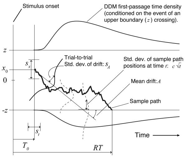
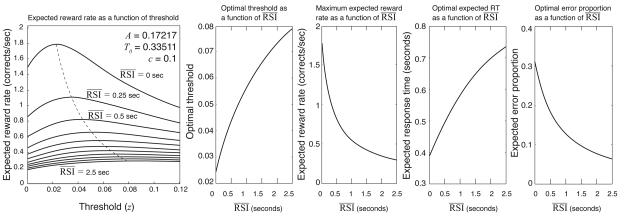
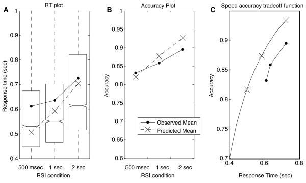
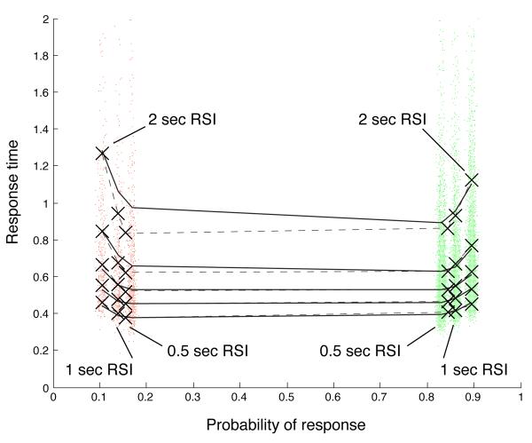
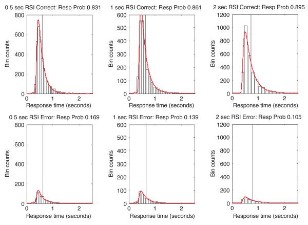
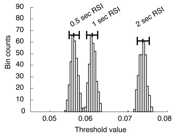
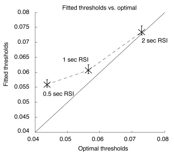
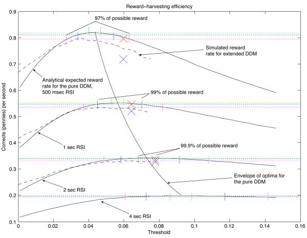
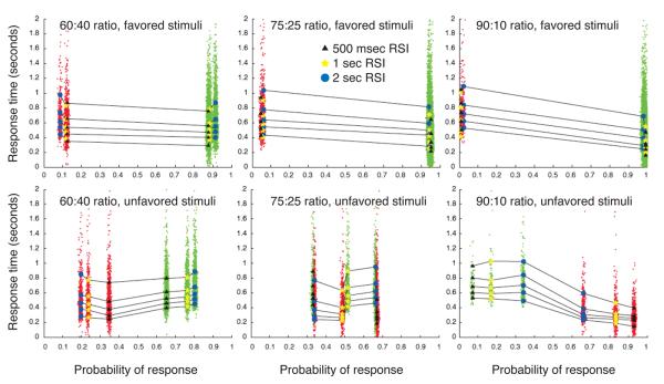
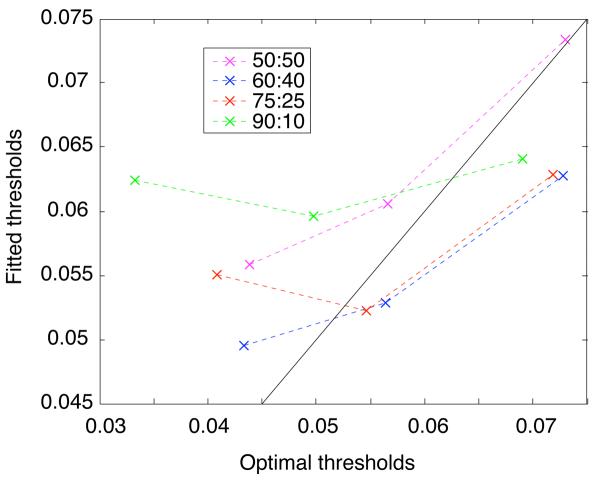
The drift-diffusion model (DDM) implements an optimal decision procedure for stationary, 2-alternative forced-choice tasks. The height of a decision threshold applied to accumulating information on each trial determines a speed-accuracy tradeoff (SAT) for the DDM, thereby accounting for a ubiquitous feature of human performance in speeded response tasks. However, little is known about how participants settle on particular tradeoffs. One possibility is that they select SATs that maximize a subjective rate of reward earned for performance. For the DDM, there exist unique, reward-rate-maximizing values for its threshold and starting point parameters in free-response tasks that reward correct responses (R. Bogacz, E. Brown, J. Moehlis, P. Holmes, & J. D. Cohen, 2006). These optimal values vary as a function of response-stimulus interval, prior stimulus probability, and relative reward magnitude for correct responses. We tested the resulting quantitative predictions regarding response time, accuracy, and response bias under these task manipulations and found that grouped data conformed well to the predictions of an optimally parameterized DDM.


Figures

Figure E1
Figure E1
Comparison of signal detection RT density to RT densities in each 2AFC condition of Experiment 2 for an individual participant, with an average RSI of 500 msec. As the stimulus proportion asymmetry increases, the RT density for two-alternative decisions approaches that for the signal detection condition.
Figure E2
Figure E2
Trial-by-trial performance data from Participant 305 in the first session of Experiment 2 (following participation in the five sessions of Experiment 1). A: Cumulative favored responses as a function of trial number. Dashed lines plot the maximum possible cumulative total of favored responses. B: RT as a function of trial number. Dashed lines indicate observed signal detection RT; superimposed solid, horizontal lines plot mean RT for the block. C: The proportion of errors within each block as a function of trial number; text indicates RSI and Π conditions in each block.
Figure E3
Figure E3
Comparison of predicted and observed response proportions, response times and error percentages in all conditions of Experiment 2, based on unconstrained, extended-DDM fits of drift and residual latency to performance of Participant 305 in Experiment 1. The horizontal axis in each plot denotes the stimulus proportions (0.6 indicates a 60:40 ratio; 0.75 indicates 75:25; 0.9 indicates 90:10). The left column of plots corresponds to a mean RSI of 500 msec; the middle column corresponds to a mean RSI of 1 sec; the right column corresponds to a mean RSI of 2 sec.
Figure F1
Figure F1
Comparison of pure DDM fits, constrained/extended DDM fits, and unconstrained/extended DDM fits in terms of harvesting efficiency. One set of reward rate curves corresponds to each of the RSI values in Experiment 1. Unconstrained/extended fits are shown in blue; constrained/extended fits in red; pure DDM fits in black.
Figure 1
Figure 1
Parameters, first-passage density and sample path for the extended drift-diffusion model (DDM). Parameters of the DDM are labeled according to the terminology of Bogacz et al. (2006); see Appendix A for a translation into the terminology of Ratcliff and colleagues (e.g., Ratcliff & Rouder, 1998).
Figure 2
Figure 2
A: Expected reward rate (RR) plotted as a function of threshold z for a range of RSI values (dashed curve connects the peaks of each RR curve). B: Optimal threshold as a function of RSI. C: RR as a function of RSI, assuming optimal thresholds at each RSI. D: Expected RT as a function of RSI, assuming optimal thresholds. E: Expected proportion of errors (ER) as a function of RSI, assuming optimal thresholds.
Figure 3
Figure 3
Critical probability surface, dividing parameter space into predicted integrative and non-integrative conditions.
Figure 4
Figure 4
Top panel: Average extended DDM parameter values from fits to 150 subsets of half the data (sampled with replacement) in each condition of Experiment 1, plotted as a function of the upper bound applied to the st and sA parameters during fitting (error bars represent the standard error of the mean). Drift A and residual latency T0 inflate as upper bounds on sA, sz and st increase, indicating a possible source of bias in parameter estimation. Bottom panel: Chi-square fit error as a function of upper bound values. Average fit-error for the bound value closest to the bounds used in our analyses was approximately 200.
Figure 5
Figure 5
A: Boxplot of response times for pooled data from all participants. Boxes represent the interquartile range (difference between first and third quartiles), and lines bisecting the boxes represent medians. Notches represent non-parametric 95% confidence intervals around the median RTs. Dashed lines and X markers indicate the expected RT predicted by Eq. 3 for a DDM with optimal thresholds, given values of A and T0 obtained from the best fit of the model to the data. Solid lines and circle markers indicate observed RT averages (these are higher than the medians indicated in the boxplots because of the skew of the RT distributions). B: Accuracy across conditions. Solid lines and circles indicate the observed proportions of correct responses. Dashed lines and X's indicate the expected proportions, 1ER, where ER in each condition is obtained by substituting fitted A and T0 values along with the optimal z value into Eq. 2. C: Predicted speed-accuracy tradeoff function (SATF) — i.e., 1ER as a function of DT+T0 — based on a fit of the DDM. Circles indicate the observed tradeoffs in each condition; X's indicate the optimal tradeoffs.
Figure 6
Figure 6
Quantile probability plot for pooled data from all participants in Experiment 1. Solid lines connect the nth quantile of the empirical data; X's and dashed lines represent the predicted quantiles for the best fit (listed in Table 1).
Figure 7
Figure 7
Group RT histograms and predicted RT densities from a fit of the DDM, sessions 4-5, Experiment 1. Columns correspond to distinct RSI conditions. The top row shows RT distributions for correct responses, while the bottom row shows the distributions of error RTs. Vertical lines indicate average RTs in each condition, computed separately for errors and corrects. Histogram bin widths were the same in both the correct and error plots for each RSI, and were determined by the Freedman-Diaconis rule (described in Appendix D).
Figure 8
Figure 8
Parametric bootstrap estimates of threshold z, showing significant differences in threshold across conditions. Horizontal whisker lines denote 95% bootstrap confidence intervals around the median threshold value.
Figure 9
Figure 9
Plot of fitted thresholds vs. optimal thresholds. Vertical crossbars indicate 95% confidence intervals around the fitted threshold values plotted as X's.
Figure 10
Figure 10
Reward harvesting efficiency of participants in three RSI conditions. One solid reward-rate curve per RSI condition represents the analytical expected reward rate for the pure DDM with the A and T0 values listed in Table 1, and with extended-DDM variability parameters set to 0. Dashed reward-rate curves show the numerical average reward rate for the extended DDM with the nonzero variability parameters listed in Table 1, simulated 10,000 times at 16 different threshold values. Green vertical lines bound intervals within which a threshold setting is expected to produce 99.9% of the maximum reward; blue lines bound 99% intervals, and magenta lines bound 97% intervals. Superimposed on these plots are blue X's denoting the fitted threshold in each condition and the observed rate of reward in each condition (total of rewards divided by total duration). Red X's correct for the penalty delays incurred by anticipatory responding, illustrating the larger proportion of anticipations in conditions with a shorter mean RSI.
Figure 11
Figure 11
Quantile probability plots for all conditions of Experiment 2. Superimposed scatterplots of RT data are plotted in green for correct responses and red for errors. Left column: 60:40 stimulus ratio. Middle column: 75:25 stimulus ratio. Right column: 90:10 stimulus ratio. The top row of panels shows quantile probability plots for responses to the more likely stimulus. The bottom row plots responses to the less likely stimulus; note the exchange of correct and error probabilities as stimulus-ratio asymmetry increases.
Figure 12
Figure 12
Fits to RT distributions in Experiment 2. Each RSI/stimulus probability condition is represented by a panel consisting of a 2 × 2 set of four plots: RTs for correct responses to favored stimuli (upper left of panel); correct responses to unfavored stimuli (upper right); errors for favored stimuli (lower left); and errors for unfavored stimuli (lower right). Three columns of these 2 × 2 plot-panels correspond to three stimulus probability conditions — 60:40, 75:25 and 90:10 stimulus odds — and three rows correspond to three RSI conditions — 500 msec, 1 sec and 2 sec.
Figure 13
Figure 13
Comparison of fitted thresholds to optimal thresholds; key identifies different stimulus-probability conditions, and the black identity line indicates what would be a perfect match. 50:50 data is from Experiment 1.
Figure 14
Figure 14
Comparison of fitted starting points to optimal starting points; key identifies different stimulus-probability conditions. 50:50 data is from Experiment 1.
Figure 15
Figure 15
Comparison of signal detection RT density to RT densities in all two-alternative forced-choice conditions of Experiment 2. Left panel: mean RSI = 500 msec. Middle panel: mean RSI = 1 sec. Right panel: mean RSI = 2 sec. As the stimulus-ratio asymmetry increases, the RT density for two-alternative decisions approaches that for the signal detection condition. This change in the RT density becomes more pronounced as the mean RSI decreases. In addition, a bimodal density appears for conditions with unequally likely stimuli, suggesting a mixture of integrative and non-integrative responding. The non-integrative modes increase in amplitude (and the integrative modes decrease) as the asymmetry in stimulus ratios increases and as the mean RSI decreases.
Figure 16
Figure 16
Comparison of predicted and observed response proportions (top row of plots), response times (middle row) and error percentages (bottom row) in all conditions of Experiment 2, based on fits of drift and residual latency. The horizontal axis in each plot denotes the stimulus proportions (0.6 indicates a 60:40 ratio; 0.75 indicates 75:25; 0.9 indicates 90:10). The left column of plots corresponds to a mean RSI of 500 msec; the middle column corresponds to a mean RSI of 1 sec; the right column corresponds to a mean RSI of 2 sec. Standard error bars are plotted, but are barely visible, in all plots.
Figure 17
Figure 17
Distribution of RTs for the favored and unfavored responses in Experiment 3, plotted against the RT distribution for signal detection obtained in Experiment 2. The RT distribution for correct favored responses is bimodal, with the earlier mode almost aligned to the maximum in the signal detection curve. The distribution of incorrect favored responses is concentrated around that early mode. Conversely, the distributions of unfavored responses show almost no sign of an early mode, and their maximum is roughly aligned with the second mode of the distribution for correct favored responses, which indicates that early responses were almost exclusively favored ones.

References

    1. Akaike H. A new look at the statistical model identification. IEEE Transactions on Automatic Control. 1974;19:716–723.
    1. Audley RJ, Pike AR. Some alternative stochastic models of choice. British Journal of Mathematical and Statistical Psychology. 1965;18:207–225.
    1. Bogacz R, Brown E, Moehlis J, Holmes P, Cohen JD. The physics of optimal decision making: a formal analysis of models of performance in two-alternative forced choice tasks. Psychological Review. 2006;113(4):700–765. - PubMed
    1. Bogacz R, Hu P, Cohen J, Holmes P. Do humans select the speed-accuracy tradeoff maximizing reward rate? in review. - PMC - PubMed
    1. Brainard DH. The psychophysics toolbox. Spatial Vision. 1997;10:433–436. - PubMed

Publication types