Experimental validation of Monte Carlo (MANTIS) simulated x-ray response of columnar CsI scintillator screens

Abstract

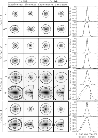
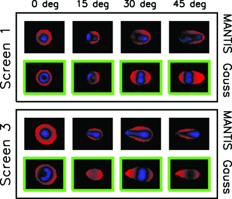
Purpose: MANTIS is a Monte Carlo code developed for the detailed simulation of columnar CsI scintillator screens in x-ray imaging systems. Validation of this code is needed to provide a reliable and valuable tool for system optimization and accurate reconstructions for a variety of x-ray applications. Whereas previous validation efforts have focused on matching of summary statistics, in this work the authors examine the complete point response function (PRF) of the detector system in addition to relative light output values.

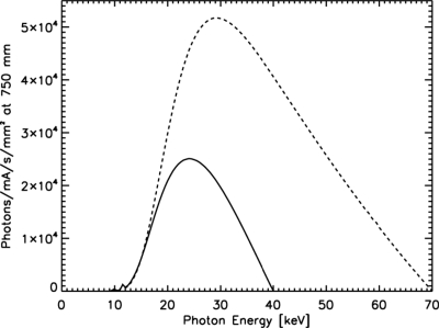
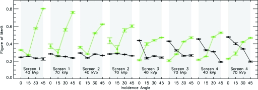
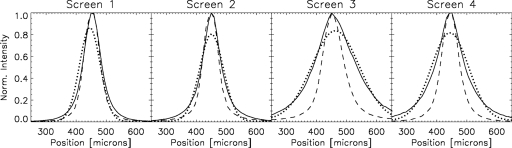
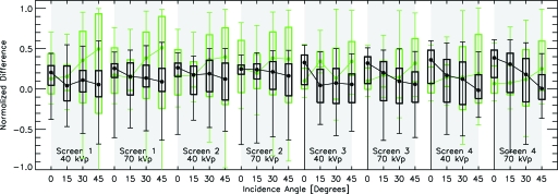
Methods: Relative light output values and high-resolution PRFs have been experimentally measured with a custom setup. A corresponding set of simulated light output values and PRFs have also been produced, where detailed knowledge of the experimental setup and CsI:Tl screen structures are accounted for in the simulations. Four different screens were investigated with different thicknesses, column tilt angles, and substrate types. A quantitative comparison between the experimental and simulated PRFs was performed for four different incidence angles (0 degrees, 15 degrees, 30 degrees, and 45 degrees) and two different x-ray spectra (40 and 70 kVp). The figure of merit (FOM) used measures the normalized differences between the simulated and experimental data averaged over a region of interest.

Results: Experimental relative light output values ranged from 1.456 to 1.650 and were in approximate agreement for aluminum substrates, but poor agreement for graphite substrates. The FOMs for all screen types, incidence angles, and energies ranged from 0.1929 to 0.4775. To put these FOMs in context, the same FOM was computed for 2D symmetric Gaussians fit to the same experimental data. These FOMs ranged from 0.2068 to 0.8029. Our analysis demonstrates that MANTIS reproduces experimental PRFs with higher accuracy than a symmetric 2D Gaussian fit to the experimental data in the majority of cases. Examination of the spatial distribution of differences between the PRFs shows that the main reason for errors between MANTIS and the experimental data is that MANTIS-generated PRFs are sharper than the experimental PRFs.

Conclusions: The experimental validation of MANTIS performed in this study demonstrates that MANTIS is able to reliably predict experimental PRFs, especially for thinner screens, and can reproduce the highly asymmetric shape seen in the experimental data. As a result, optimizations and reconstructions carried out using MANTIS should yield results indicative of actual detector performance. Better characterization of screen properties is necessary to reconcile the simulated light output values with experimental data.

Figure 1

Schematic of CCD setup with a 30° pinhole holder (not to scale). Diverging x rays enter from the right. The pinhole is mounted in a caphead screw and positioned in an aluminum holder at the desired angular orientation. Lead lining within the aluminum holder provides shielding from background signal and has a hole oriented to allow the primary signal through. The signal then passes through a Be window and compressed foam before impacting the screen and producing the optical signal that travels down the FOP to the optical detector. A cross-sectional view (not to scale) of the pinhole disk is shown in the inset (Ref. 16). The manufacturer specifies L=75±10 μm and D=30±5 μm for the 30 μm pinhole. Note that, when drawn to scale, the size of the straight edged portion of the pinhole is much smaller than the angled opening.

Figure 2

SEM measurements of all screens. The physical size of the white scale bar at the bottom of each SEM as well as the magnification are given following the screen number. (a) Screen 1 (77.4 μm, 200×), (b) screen 2 (56.44 μm, 300×), (c) screen 3 (151.36 μm, 100×), and (d) screen 4 (151.36 μm, 100×)

Figure 3

Spectra used in MANTIS simulations of the experimental PRFs: 40 kVp (solid line) and 70 kVp (dashed line). Both spectra include 1.0 mm Al filtration.

Figure 4

(left) SEM of screen 1 (white scale bar = 77.4 μm, magnification =200×) (right) Schematic of MANTIS model of the same screen (to scale). The thin layer at the top of the image represents the organic polymer. The organic polymer layer is followed by the columnar zone, where light gray indicates CsI and dark gray is the intercolumnar space. The next layer is the homogeneous CsI and, finally, the bottom layer is the substrate.

Figure 5

Experimental and simulated PRFs for screens 1–4. (first column) 40 kVp, experimental (second column) 40 kVp, simulations from MANTIS (third column) 70 kVp, experimental (fourth column) 70 kVp, simulations from MANTIS (fifth column) 40 kVp, horizontal cuts through the center of the PRFs, experimental data are shown with a solid line and MANTIS results are shown as a dashed line. The different screens are labeled as well as the incidence angles. Only incidence angles of 0° and 45° are shown. Contour lines shown on the plots are for levels of 0.01, 0.05, and 0.1 (the maximum is always 1). All PRFs are 101 × 101 pixels with 9 μm∕pixel.

Figure 6

FOMs for all screens, energies, and incidence angles. Black indicates the results from the comparison of experimental data with MANTIS-generated PRFs and green indicates the results from the comparison with a 2D symmetric Gaussian fit to the zero-angle experimental data. The values displayed are means of FOMs calculated from 11 independent experimental and simulated images, while the error bars represent the standard deviation of those 11 different FOMs.

Figure 7

Comparison of experimental, MANTIS, and Gaussian fit PRFs at zero degrees for 40 kVp. One-dimensional, horizontal cuts through the center of the PRFs are shown for each screen. The experimental data are shown as a solid line, MANTIS as a dashed line, and the Gaussian fits as a dotted line. We can see in all cases that the Gaussian fit underestimates the peak of the PRF. For the thicker screens (screens 3 and 4), MANTIS provides a much sharper PRF than the experimental data and, as a result, the FOM calculation indicates a better match to the experimental data for the Gaussian fit than MANTIS.

Figure 8

The normalized difference of the PRFs is plotted as a function of incidence angle for all screens, energies, and incidence angles. Normalized differences from the comparison with MANTIS are plotted in black, while normalized differences from the 2D Gaussian fit are plotted in green. The box plots show the median normalized difference (in the ROI) as the filled circle, the bottom and top of the box are the first and third quartiles, and the bottom and top error bars show the minimum and maximum normalized differences.

Figure 9

Images showing the spatial distribution of the normalized differences for all incidence angles of screens 1 and 3 with the 40 kVp spectrum. Images from the comparison of experimental data with MANTIS are outlined in black and labeled “MANTIS,” while images from the comparison with the 2D Gaussian fit are outlined in a green box and labeled “Gauss.” Negative normalized differences are mapped to shades of blue, positive to shades of red, and zero to black. The images are all scaled to have red, blue, and black as corresponding to the most positive, most negative, and zero data values, respectively. As a result, these images simply indicate the spatial location and relative magnitude of differences and not the absolute magnitude of the difference which is indicated in Fig. 8.

References

-
- Jing T., Goodman C. A., Drewery J., Cho G., Hong W. S., Lee H., Kaplan S. N., Mireshghi A., Perez-Mendez V., and Wildermuth D., “Amorphous silicon pixel layers with cesium iodide converters for medical radiography,” IEEE Trans. Nucl. Sci. IETNAE 41(4), 903–909 (1994).10.1109/23.322829 - DOI
- Nagarkar V. V., Gupta T. K., Miller S. R., Klugerman Y., Squillante M. R., and Entine G., “Structured CsI(Tl) scintillators for x-ray imaging applications,” IEEE Trans. Nucl. Sci. IETNAE 45(3), 492–496 (1998).10.1109/23.682433 - DOI
Publication types
MeSH terms
Substances
Grants and funding
LinkOut - more resources
Full Text Sources
Medical
Research Materials