Global sea level linked to global temperature

Abstract

We propose a simple relationship linking global sea-level variations on time scales of decades to centuries to global mean temperature. This relationship is tested on synthetic data from a global climate model for the past millennium and the next century. When applied to observed data of sea level and temperature for 1880-2000, and taking into account known anthropogenic hydrologic contributions to sea level, the correlation is >0.99, explaining 98% of the variance. For future global temperature scenarios of the Intergovernmental Panel on Climate Change's Fourth Assessment Report, the relationship projects a sea-level rise ranging from 75 to 190 cm for the period 1990-2100.

Fig. 1.

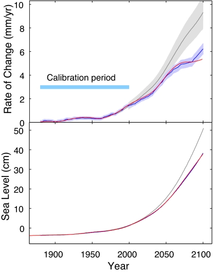
The 21st-century simulation. (Upper) The rate of sea-level rise from a climate model simulation (red) compared with that predicted by Eq. 1 (gray) and Eq. 2 (blue) based on global mean temperature from the climate model. Shaded areas show the uncertainty of the fit (1 SD). The parameter calibration period is 1880–2000, and 2000–2100 is the validation period. (Lower) The integral of the curves in Upper, i.e., sea-level proper.

Fig. 2.

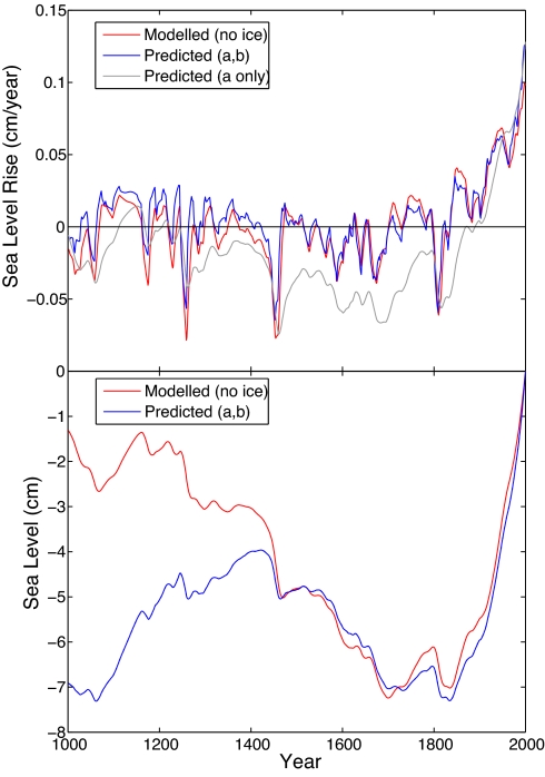
The millennnium simulation. (Upper) Rate of sea-level rise for the last millennium from a climate model simulation (red), compared with that predicted by Eq. 1 (gray) and Eq. 2 (blue) based on global mean temperature from the climate model. Note that parameter calibration was done for the model simulation shown in Fig. 1 for 1880–2000 only (but see below for T₀). (Lower) Sea level for the last millennium, obtained by integration. A correction to the T₀ parameter of −0.13 K (corresponding to a constant sea-level trend of a·T₀ = −0.1 mm/year) was applied to make the long-term sea-level trends match better after the year 1400.

Fig. 3.

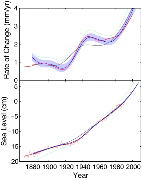
The duel model in the instrumental period. (Upper) Observations-based rate of sea-level rise (with tectonic and reservoir effects removed; red) compared with that predicted by Eq. 1 (gray) and Eq. 2 (blue with uncertainty estimate) using observed global mean temperature data. Also shown is the estimate from Eq. 2 using only the first half of the data (green) or the second half of the data (light blue). (Lower) The integral of the curves in Upper, i.e., sea-level proper. In addition to the smoothed sea level used in the calculations, the annual sea-level values (thin red line) are also shown. The dark blue prediction by Eq. 2 almost obscures the observed sea level because of the close match.

Fig. 4.

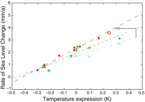
Blue crosses show 15-year averages of global temperature (relative to 1951–1980) versus the rate of sea-level rise, with their linear least-squares fit, as in R07 (3) but using 15-year bins. The green crosses show the adjustment to sea level induced by the reservoir correction (22), leading to a steeper slope. The red dots show the expression (T + b/a dT/dt) appearing on the right of Eq. 2. This increases the slope again and leads to a much tighter linear fit. The open red circle is a data point based on the satellite altimetry data for 1993–2008. The arrow indicates how the linear trend line changes from that of R07 (blue) to the green one by adjusting the sea-level data (a change along the vertical axis) and then again to the red line by adjusting the temperature expression (along the horizontal axis).

Fig. 5.

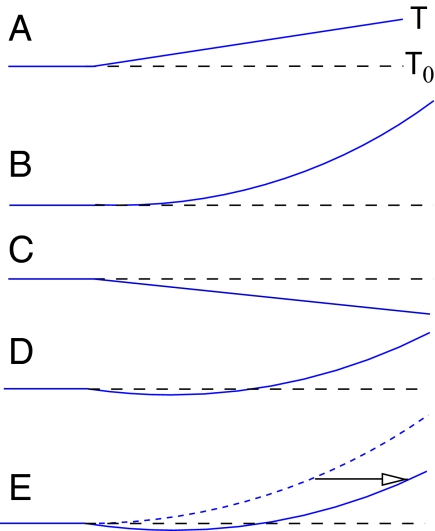
Schematic of the response to a linear temperature rise. (A) Temperature. (B) First term on the right of Eq. 2. (C) Second term. (D) Total sea-level response. (E) Comparison to the case b = 0 (Eq. 1), showing that b < 0 primarily corresponds to a time lag in the sea-level response.

Fig. 6.

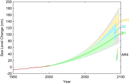
Projection of sea-level rise from 1990 to 2100, based on IPCC temperature projections for three different emission scenarios (labeled on right, see Projections of Future Sea Level for explanation of uncertainty ranges). The sea-level range projected in the IPCC AR4 (2) for these scenarios is shown for comparison in the bars on the bottom right. Also shown is the observations-based annual global sea-level data (18) (red) including artificial reservoir correction (22).

References

-
- Rahmstorf S, et al. Recent climate observations compared to projections. Science. 2007;316:709. - PubMed
- Solomon S, et al., editors. Intergovernmental Panel on Climate Change. The Fourth Assessment Report of the Intergovernmental Panel on Climate Change. Cambridge UK: Cambridge Univ Press; 2007.
- Rahmstorf S. A semiempirical approach to projecting future sea-level rise. Science. 2007;315:368–370. - PubMed
- Horton R, et al. Sea-level rise projections for current generation CGCMs based on the semiempirical method. Geophys Res Lett. 2008;35:L02715.
- Edwards R. Sea levels: Resolution and uncertainty. Progr Phys Geogr. 2007;31:621–632.
LinkOut - more resources
Full Text Sources
Miscellaneous