Comparative Study
. 2009 Dec 16;29(50):15780-95.
doi: 10.1523/JNEUROSCI.2305-09.2009.

Cooperative and competitive interactions facilitate stereo computations in macaque primary visual cortex

Affiliations
Comparative Study

Cooperative and competitive interactions facilitate stereo computations in macaque primary visual cortex

Jason M Samonds et al. J Neurosci. .

Abstract

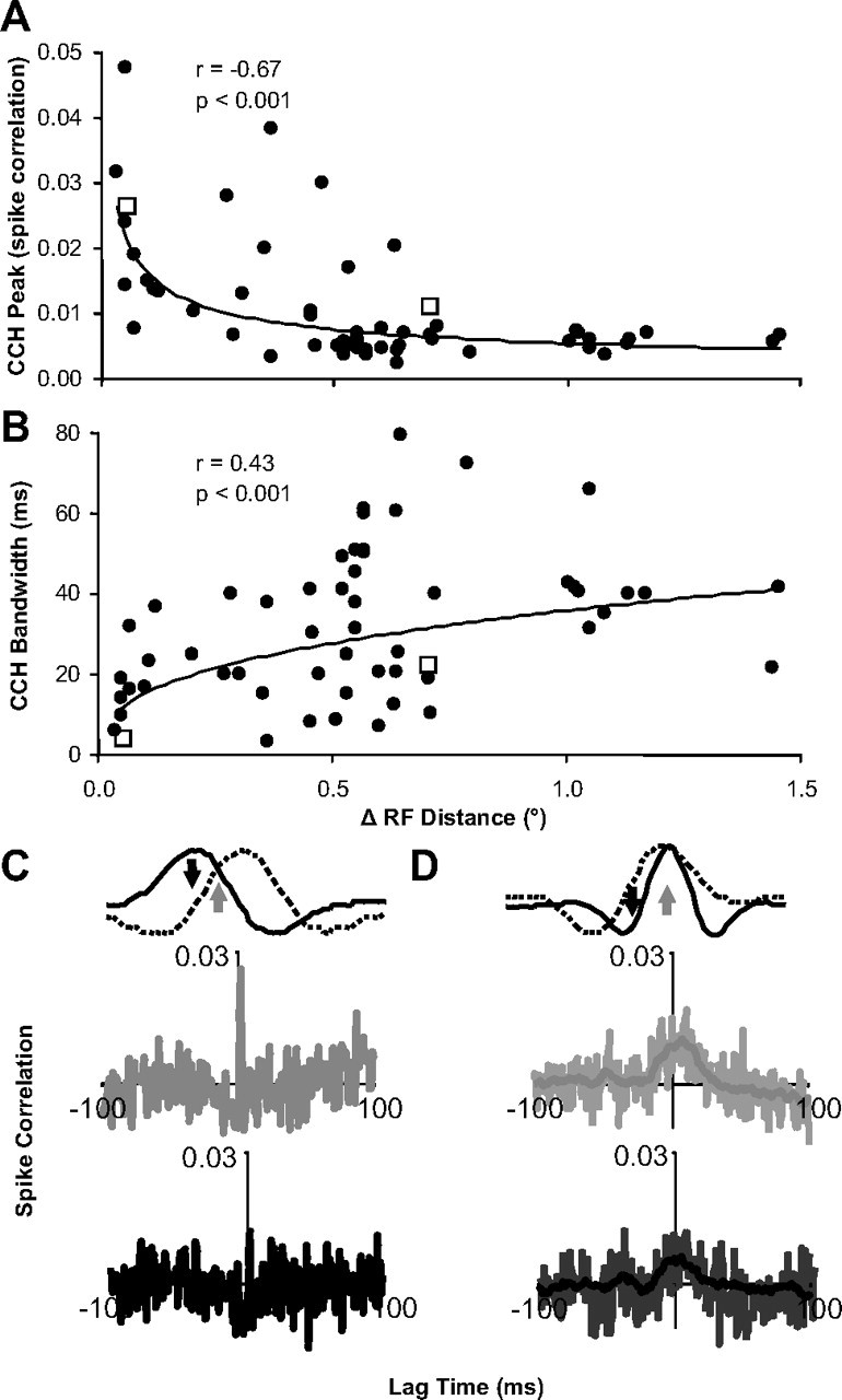
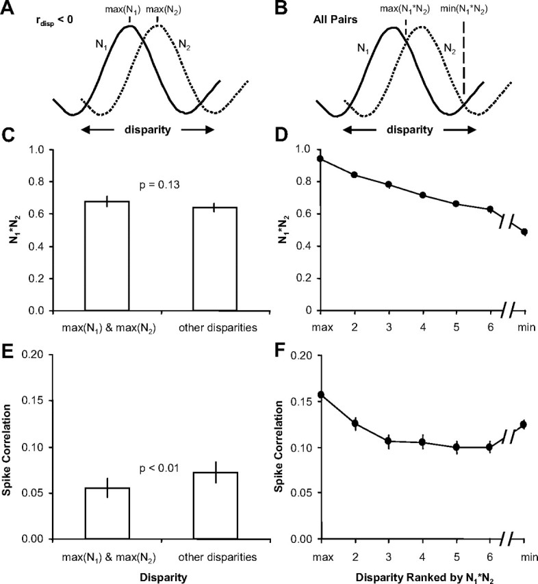
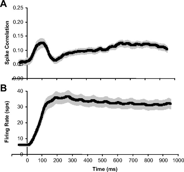
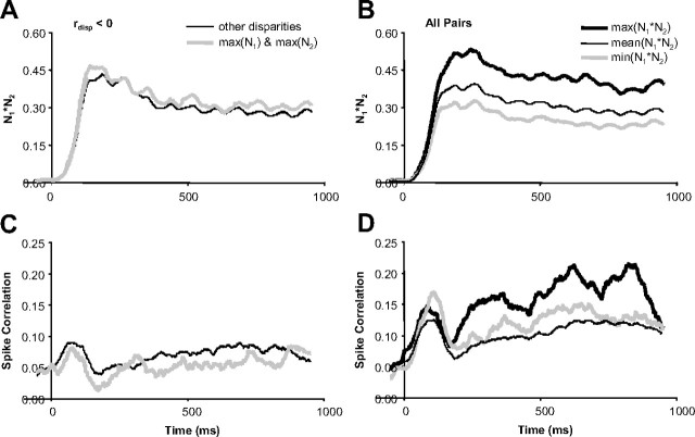
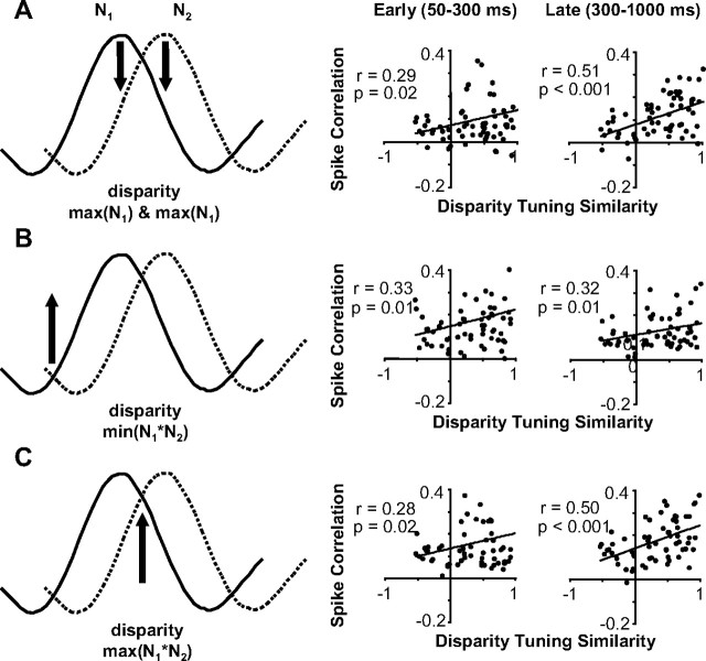
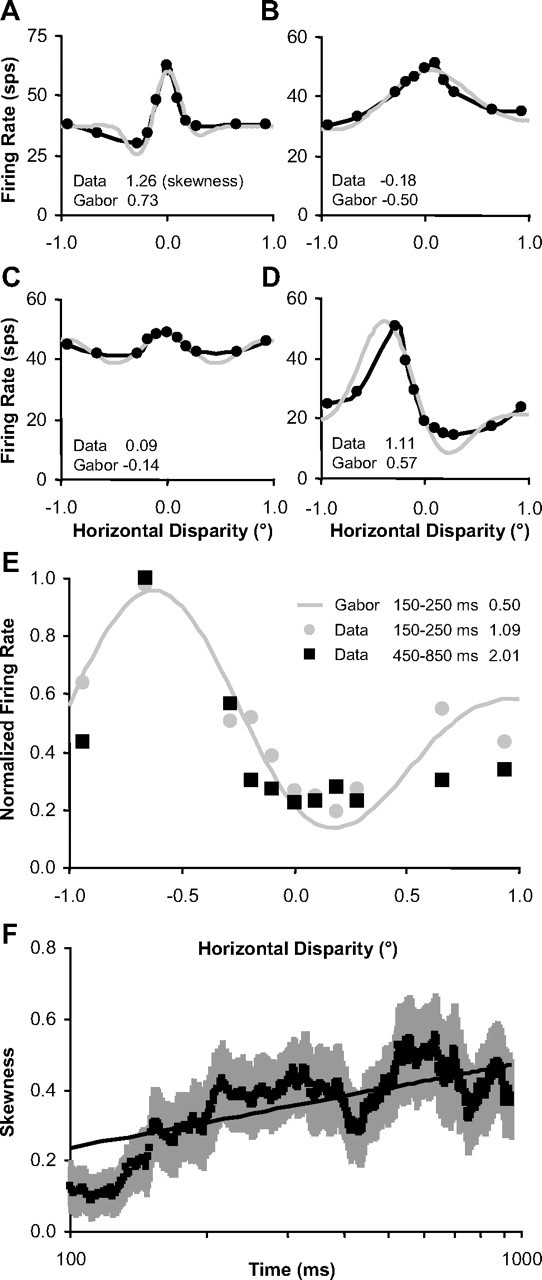
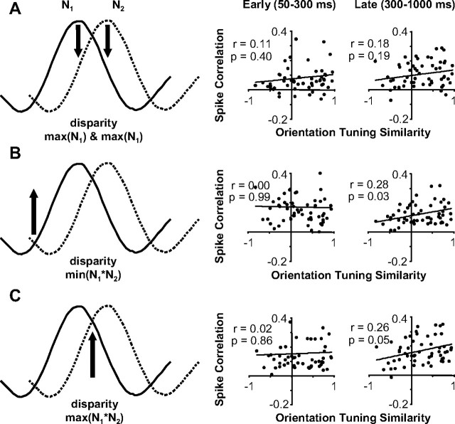
Inferring depth from binocular disparities is a difficult problem for the visual system because local features in the left- and right-eye images must be matched correctly to solve this "stereo correspondence problem." Cortical architecture and computational studies suggest that lateral interactions among neurons could help resolve local uncertainty about disparity encoded in individual neurons by incorporating contextual constraints. We found that correlated activity among pairs of neurons in primary visual cortex depended both on disparity-tuning relationships and the stimuli displayed within the receptive fields of the neurons. Nearby pairs of neurons with distinct disparity tuning exhibited a decrease in spike correlation at competing disparities soon after response onset. Distant neuronal pairs of similar disparity tuning exhibited an increase in spike correlation at mutually preferred disparities. The observed correlated activity and response dynamics suggests that local competitive and distant cooperative interactions improve disparity tuning of individual neurons over time. Such interactions could represent a neural substrate for the principal constraints underlying cooperative stereo algorithms.


Figures

Figure 1.
Figure 1.
A, B, An example recording session. In this session, we used three dual electrode microdrives in a 2 × 3 configuration (one electrode failed to record neural activity and was disconnected). A, Position of the six-electrode array with respect to the macaque brain and the grid where microdrives were attached within the recording chamber (dashed lines are approximate retinotopic coordinates and solid black line overlaying the grid is approximate location of the lunate sulcus based on several previous recording sessions within this chamber). The bottom plots show filtered neural activity for all channels and samples of triggered and on-line sorted action potentials. B, Receptive field locations (minimum response field) with respect to fixation (red) and DRDS stimulation. C, D, Examples of multiple waveforms (dotted lines are SDs) recorded on the same electrode. C, We typically encountered multiple units that were easily distinguishable (these are waveforms for the competitive example pair of neurons described in the main text). D, The most waveform overlap that was allowed to consider multiple waveforms on the same electrode for cross-correlation analysis.
Figure 2.
Figure 2.
A, B, Population average of normalized CCHs (n = 63 pairs, centered on their peak). The dotted lines are population average of individual pairs' 95% confidence intervals (n = 60 trials). A, Raw cross-covariance derived CCH (red) versus excitability corrected and bootstrapped CCH (blue). B, Shift-predictor CCH (red) versus excitability corrected and bootstrapped CCH (blue). C, Population average CCH (blue) and chance correlation (red). D, Zoomed-in plot of chance correlation. E, Example CCH for DRDS modulated at 12 or 7 Hz (dashed lines are bootstrapped 95% confidence interval; n = 60 trials).
Figure 3.
Figure 3.
Evidence of competitive and cooperative interaction. A, Neurons with overlapping receptive fields that were presented random dot stereograms (only the image for one eye is shown). The white squares and bars are preferred orientation and direction of motion. The red square is fixation point. B, Disparity tuning for neurons in A. C, Correlation versus time (100 ms sliding windows) for same data shown in B (averaged over all disparities). D, Neurons with neighboring receptive fields. E, Disparity tuning for neurons in D. F, Correlation versus time for same data shown in E (averaged over all disparities). All error bars are trial-to-trial SE (n = 60).
Figure 4.
Figure 4.
Relationship between receptive field distance and disparity-tuning similarity for neuronal pairs that exhibit spike correlation (n = 63 pairs). Scatter plot of the distance between receptive field centers versus disparity-tuning similarity for each pair of neurons. The open squares are examples from Figure 3.
Figure 5.
Figure 5.
Distance and stimulus dependence of spike correlation properties. A, Scatter plot of the CCH peak height versus distance between receptive field centers for each pair of neurons (n = 63 pairs; power fit). B, Scatter plot of the CCH peak width (half-height) versus distance between receptive field centers for each pair of neurons (n = 63 pairs; power fit). C, D, Example CCHs (A, B, open squares) for overlapping and neighboring receptive fields, respectively, when a disparity was presented that led to a strong response for both neurons (gray) and a stronger response in one neuron relative to the other neuron (black) (n = 60 trials). In D, the light lines in each CCH plot are raw estimates, and the darker lines are smoothed data that were used for any analysis described in the article.
Figure 6.
Figure 6.
Spike correlation depended on the disparity presented. A, Spike correlation and N1*N2 were compared between preferred and nonpreferred disparities. B, Spike correlation and N1*N2 were computed for all disparities and ranked by N1*N2. Only 7 disparities are shown, because only 7 of the 11 disparities were presented for some pairs of neurons. C, Population average (n = 17 pairs) of N1*N2 for the maximum of N1 and N2 and all other disparities. D, Population average (n = 63 pairs) of N1*N2 sorted by the disparity presented that caused the maximum (max) to the minimum (min) response. E, Population average of spike correlation measurements for the corresponding data presented in C. F, Population average of spike correlation measurements for the corresponding data presented in D. Error bars are population SE.
Figure 7.
Figure 7.
Spike correlation varies over time during stimulation. A, Population average of spike correlation versus time (sliding 100 ms windows). B, Population average of firing rate versus time (sliding 100 ms windows). All error bars are population SE (n = 63 neurons). Data for each neuron averaged over all disparities are presented.
Figure 8.
Figure 8.
Timing of spike correlation depended on the disparity presented. A, Population average (n = 17 pairs) of N1*N2 versus time for the maximum of N1 and N2 and all other disparities. B, Population average (n = 63 pairs) of maximum, mean, and minimum N1*N2 versus time. C, Population average of spike correlation versus time for the corresponding data presented in A. D, Population average of spike correlation versus time for the corresponding data presented in B.
Figure 9.
Figure 9.
The relationship between spike correlation and disparity-tuning similarity considering disparity presented and response latency. A, Data for all neuronal pairs when a preferred disparity was presented (maximum of N1 and N2). Scatter plots of spike correlation versus disparity-tuning similarity for early (50–300 ms; left) and late (300–1000 ms; right) period of stimulation. B, Same organization as A, but for data when the common least preferred disparity was presented (minimum of N1*N2). C, Same organization as A, but for data when the common most preferred disparity was presented (maximum of N1*N2). All regression analysis was based on n = 63 pairs.
Figure 10.
Figure 10.
Disparity tuning improved over time (examples). A, D, G, J, Examples of firing rates over time for preferred and progressively less preferred disparities. B, E, H, K, Disparity-tuning curves of same example neurons computed at progressively later intervals from stimulus onset (Gabor fits). C, F, I, L, Tuning curves of same example neurons ranked from the disparity presented that caused the strongest (best) to the weakest (worst) response (linear, log, and power fits). Note that the vertical axis is the same between the center and right column (peak-normalized firing rate). All average firing rates are based on n = 60 trials.
Figure 11.
Figure 11.
Disparity tuning improved over time (population statistics). A, Population average of firing rate over time for preferred and progressively less preferred disparities. B, Population average of disparity tuning computed at progressively later intervals from stimulus onset (normalized by the peak response in each interval). C, Population average of the slopes computed by linear, log, and power fits of ranked disparity responses over time (rank determined over entire stimulation period). D, Scatter plot of slopes computed at progressively later intervals versus slopes computed during the initial interval. Error bars are population SE (n = 60 neurons).
Figure 12.
Figure 12.
Temporal dynamics of disparity-tuning curve peaks and valleys. A, Schematic of the tuning curve features examined over time. B, Population average of firing rates at the points on the tuning curve described in A (time axis is plotted in log scale). C, Population average of the ratio of firing rates: (peak − valley)/(peak + valley). D, Population average of the ratio of firing rates: (peak − valley)/(SD of the tuning curve). Error bars are population SE (n = 52 neurons), and straight lines are logarithmic regression fit.
Figure 13.
Figure 13.
Disparity-tuning skewness increased over time. A–D, Examples of disparity-tuning curves (black) that deviate from fitted Gabor functions (gray). Skewness values for data and Gabor fits are listed in the bottom left corner of each plot. E, Example taken from Figure 10K to demonstrate increasing skewness with respect to time (skewness listed on the right side of the legend). F, Population average of skewness versus time for n = 24 neurons with the most robust disparity tuning (see text). Error bars are population SE, and straight line is logarithmic regression fit.
Figure 14.
Figure 14.
The relationship between spike correlation and orientation-tuning similarity considering disparity presented and response latency (during DRDS presentation). A, Data for all neuronal pairs when a preferred disparity was presented (maximum of N1 and N2). Scatter plots of spike correlation versus orientation-tuning similarity for early (50–300 ms; left) and late (300–1000 ms; right) period of stimulation. B, Same organization as A, but for data when the common least preferred disparity was presented (minimum of N1*N2). C, Same organization as A, but for data when the common most preferred disparity was presented (maximum of N1*N2). All regression analysis was based on n = 63 pairs.

Similar articles

Cited by

References

    1. Aertsen AM, Gerstein GL, Habib MK, Palm G. Dynamics of neuronal firing correlation: modulation of “effective connectivity.”. J Neurophysiol. 1989;61:900–917. - PubMed
    1. Angelucci A, Bullier J. Reaching beyond the classical receptive field of V1 neurons: horizontal or feedback axons? J Physiol Paris. 2003;97:141–154. - PubMed
    1. Bair W, Zohary E, Newsome WT. Correlated firing in macaque visual area MT: time scales and relationship to behavior. J Neurosci. 2001;21:1676–1697. - PMC - PubMed
    1. Ben-Shahar O, Huggins PS, Izo T, Zucker SW. Cortical connections and early visual function: intra- and inter-columnar processing. J Physiol Paris. 2003;97:191–208. - PubMed
    1. Bosking WH, Zhang Y, Schofield B, Fitzpatrick D. Orientation selectivity and the arrangement of horizontal connections in tree shrew striate cortex. J Neurosci. 1997;17:2112–2127. - PMC - PubMed

Publication types