

Pinna cues determine orienting response modes to synchronous sounds in elevation
- PMID: 20053901
- PMCID: PMC6632510
- DOI: 10.1523/JNEUROSCI.2982-09.2010
Pinna cues determine orienting response modes to synchronous sounds in elevation
Abstract
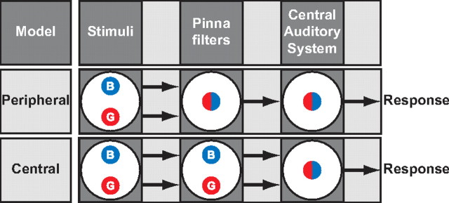
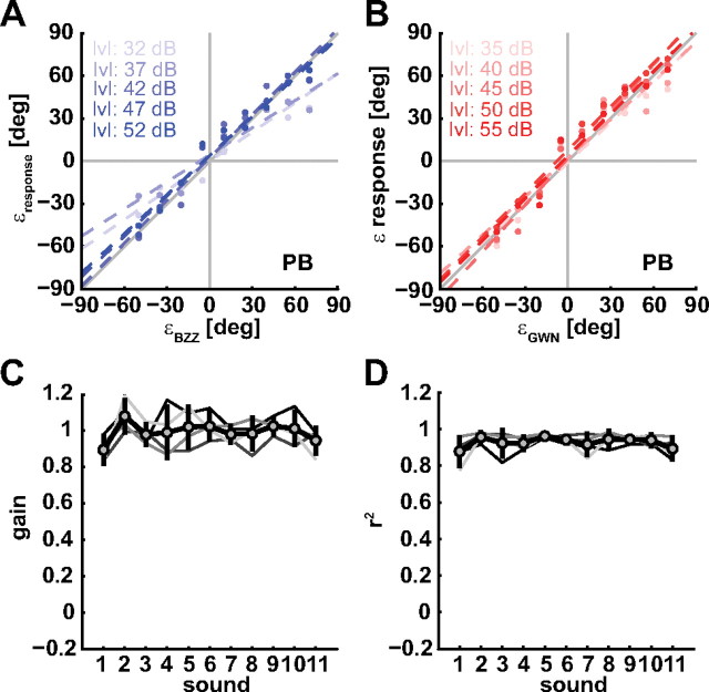
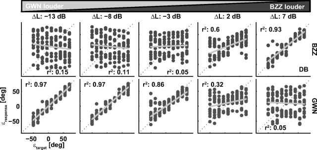
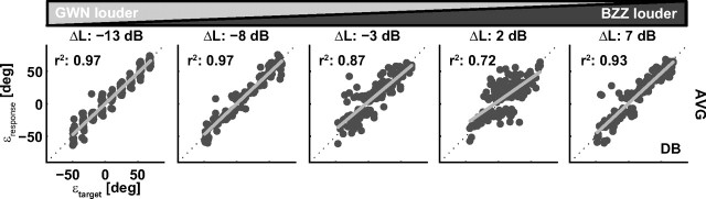
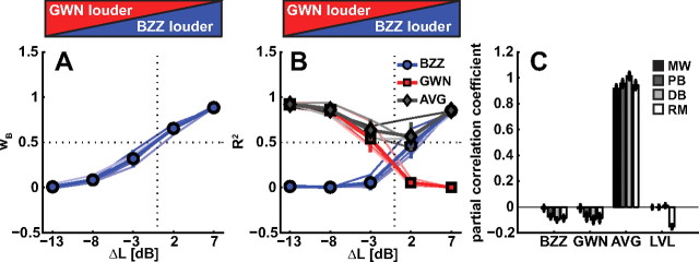
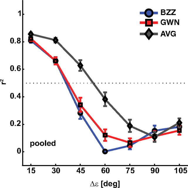
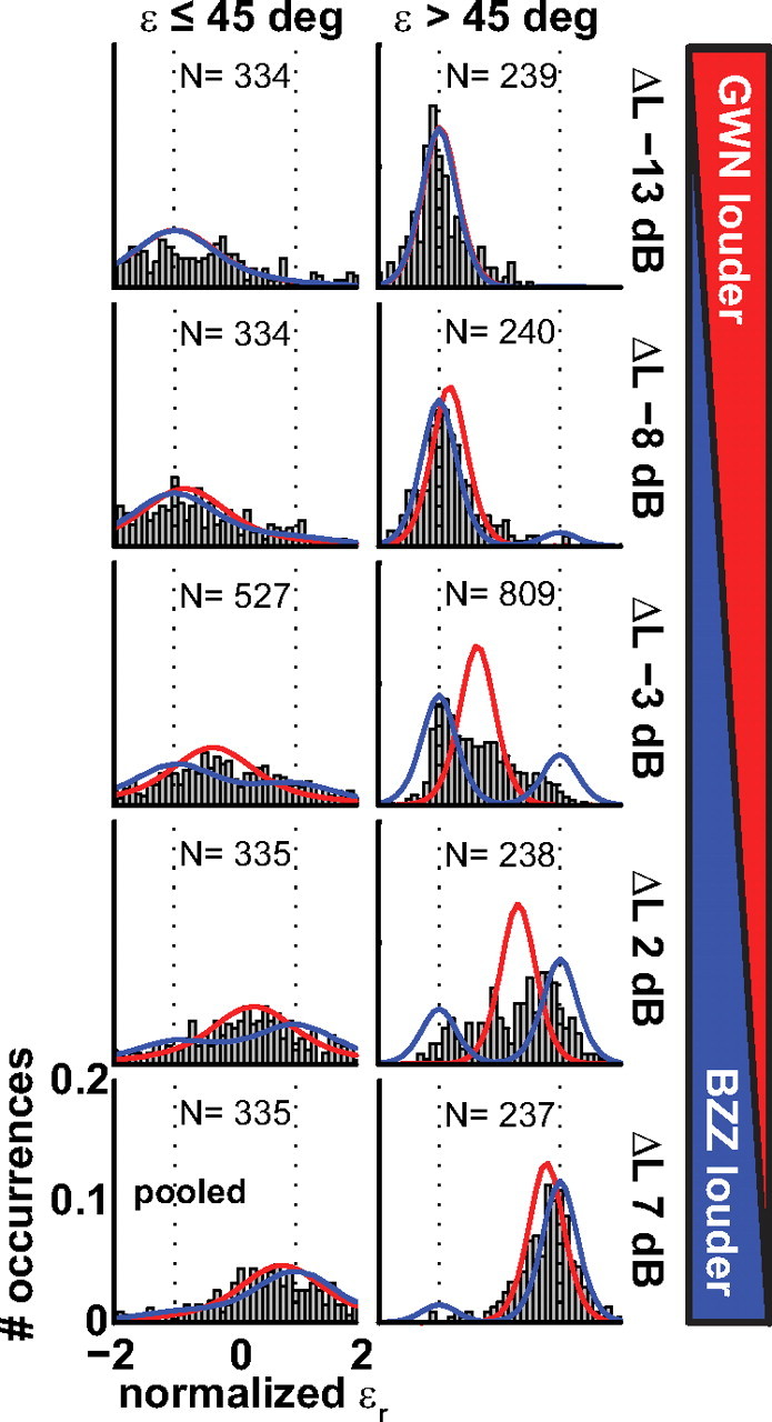
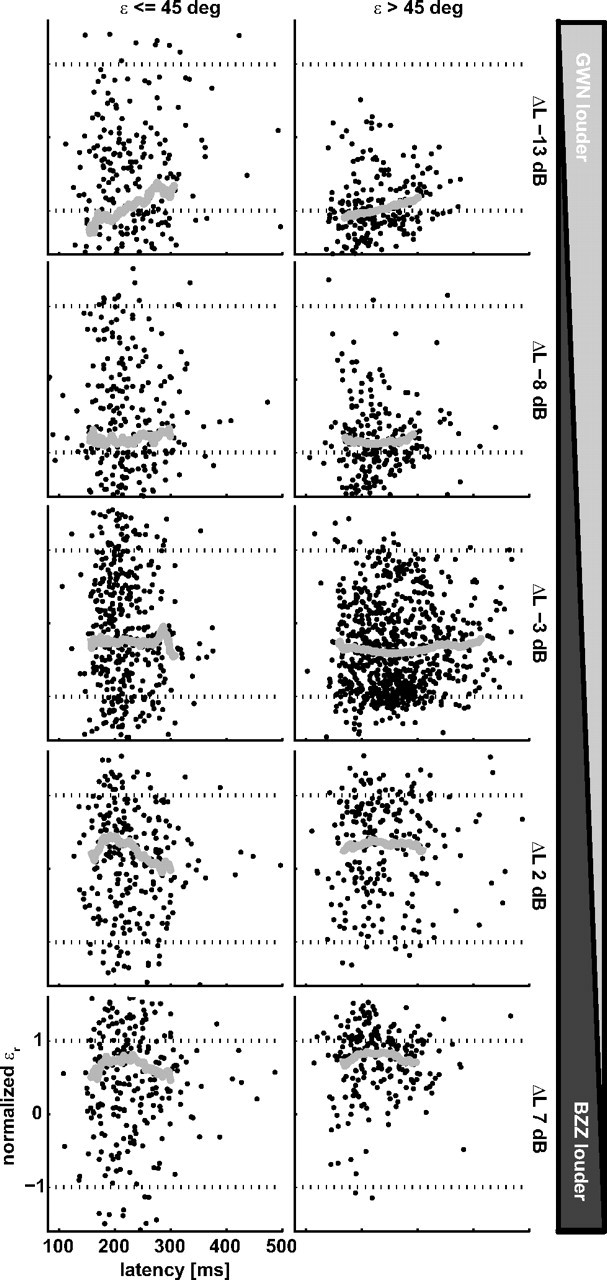
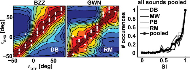
To program a goal-directed orienting response toward a sound source embedded in an acoustic scene, the audiomotor system should detect and select the target against a background. Here, we focus on whether the system can segregate synchronous sounds in the midsagittal plane (elevation), a task requiring the auditory system to dissociate the pinna-induced spectral localization cues. Human listeners made rapid head-orienting responses toward either a single sound source (broadband buzzer or Gaussian noise) or toward two simultaneously presented sounds (buzzer and noise) at a wide variety of locations in the midsagittal plane. In the latter case, listeners had to orient to the buzzer (target) and ignore the noise (nontarget). In the single-sound condition, localization was accurate. However, in the double-sound condition, response endpoints depended on relative sound level and spatial disparity. The loudest sound dominated the responses, regardless of whether it was the target or the nontarget. When the sounds had about equal intensities and their spatial disparity was sufficiently small, endpoint distributions were well described by weighted averaging. However, when spatial disparities exceeded approximately 45 degrees, response endpoint distributions became bimodal. Similar response behavior has been reported for visuomotor experiments, for which averaging and bimodal endpoint distributions are thought to arise from neural interactions within retinotopically organized visuomotor maps. We show, however, that the auditory-evoked responses can be well explained by the idiosyncratic acoustics of the pinnae. Hence basic principles of target representation and selection for audition and vision appear to differ profoundly.
Figures

Similar articles
-
Influence of head position on the spatial representation of acoustic targets.J Neurophysiol. 1999 Jun;81(6):2720-36. doi: 10.1152/jn.1999.81.6.2720. J Neurophysiol. 1999. PMID: 10368392
-
Level-weighted averaging in elevation to synchronous amplitude-modulated sounds.J Acoust Soc Am. 2017 Nov;142(5):3094. doi: 10.1121/1.5011182. J Acoust Soc Am. 2017. PMID: 29195479 Free PMC article.
-
Spatiotemporal factors influence sound-source segregation in localization behavior.J Neurophysiol. 2021 Feb 1;125(2):556-567. doi: 10.1152/jn.00184.2020. Epub 2020 Dec 30. J Neurophysiol. 2021. PMID: 33378250 Free PMC article.
-
Evidence for a vestigial pinna-orienting system in humans.Psychophysiology. 2015 Oct;52(10):1263-70. doi: 10.1111/psyp.12501. Epub 2015 Jul 24. Psychophysiology. 2015. PMID: 26211937 Review.
-
Behavioral studies of sound localization in the cat.J Neurosci. 1998 Mar 15;18(6):2147-60. doi: 10.1523/JNEUROSCI.18-06-02147.1998. J Neurosci. 1998. PMID: 9482800 Free PMC article. Review.
Cited by
-
Age-related hearing loss and ear morphology affect vertical but not horizontal sound-localization performance.J Assoc Res Otolaryngol. 2013 Apr;14(2):261-73. doi: 10.1007/s10162-012-0367-7. Epub 2013 Jan 15. J Assoc Res Otolaryngol. 2013. PMID: 23319012 Free PMC article.
-
Temporal Cortex Activation to Audiovisual Speech in Normal-Hearing and Cochlear Implant Users Measured with Functional Near-Infrared Spectroscopy.Front Hum Neurosci. 2016 Feb 11;10:48. doi: 10.3389/fnhum.2016.00048. eCollection 2016. Front Hum Neurosci. 2016. PMID: 26903848 Free PMC article.
-
Modeling Localization of Amplitude-Panned Virtual Sources in Sagittal Planes.J Audio Eng Soc. 2015 Aug 18;63(7-8):562-569. doi: 10.17743/jaes.2015.0063. J Audio Eng Soc. 2015. PMID: 26441471 Free PMC article.
-
Atypical vertical sound localization and sound-onset sensitivity in people with autism spectrum disorders.J Psychiatry Neurosci. 2013 Nov;38(6):398-406. doi: 10.1503/jpn.120177. J Psychiatry Neurosci. 2013. PMID: 24148845 Free PMC article.
-
Testing the Precedence Effect in the Median Plane Reveals Backward Spatial Masking of Sound.Sci Rep. 2018 Jun 6;8(1):8670. doi: 10.1038/s41598-018-26834-2. Sci Rep. 2018. PMID: 29875363 Free PMC article.
References
-
- Aitsebaomo AP, Bedell HE. Saccadic and psychophysical discrimination of double targets. Optom Vis Sci. 2000;77:321–330. - PubMed
-
- Algazi R, Duda RO, Thompson DM, Avendano C. The CIPIC HRTF database. Paper presented at 2001 IEEE Workshop on Applications of Signal Processing to Audio and Electroacoustics; October; New Paltz, NY. 2001.
-
- Arai K, McPeek RM, Keller EL. Properties of saccadic responses in monkey when multiple competing visual stimuli are present. J Neurophysiol. 2004;91:890–900. - PubMed
-
- Becker W, Jürgens R. An analysis of the saccadic system by means of double step stimuli. Vision Res. 1979;19:967–983. - PubMed
-
- Best V, van Schaik A, Carlile S. Separation of concurrent broadband sound sources by human listeners. J Acoust Soc Am. 2004;115:324–336. - PubMed
Publication types
MeSH terms
LinkOut - more resources
Full Text Sources