Functional, but not anatomical, separation of "what" and "when" in prefrontal cortex

Abstract

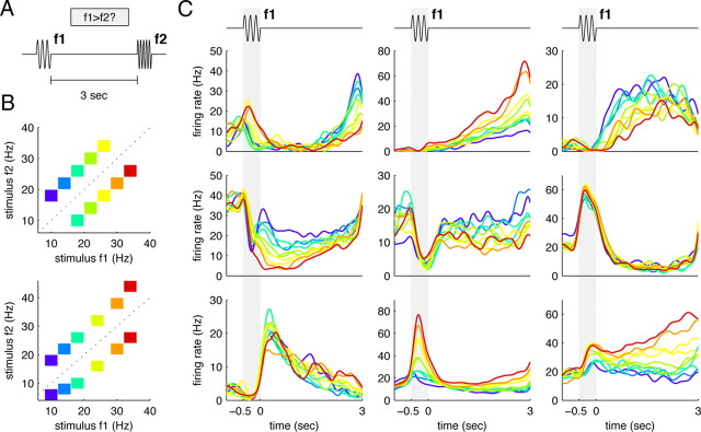
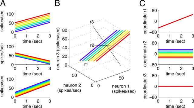
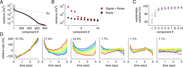
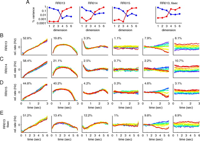
How does the brain store information over a short period of time? Typically, the short-term memory of items or values is thought to be stored in the persistent activity of neurons in higher cortical areas. However, the activity of these neurons often varies strongly in time, even if time is unimportant for whether or not rewards are received. To elucidate this interaction of time and memory, we reexamined the activity of neurons in the prefrontal cortex of monkeys performing a working memory task. As often observed in higher cortical areas, different neurons have highly heterogeneous patterns of activity, making interpretation of the data difficult. To overcome these problems, we developed a method that finds a new representation of the data in which heterogeneity is much reduced, and time- and memory-related activities became separate and easily interpretable. This new representation consists of a few fundamental activity components that capture 95% of the firing rate variance of >800 neurons. Surprisingly, the memory-related activity components account for <20% of this firing rate variance. The observed heterogeneity of neural responses results from random combinations of these fundamental components. Based on these components, we constructed a generative linear model of the network activity. The model suggests that the representations of time and memory are maintained by separate mechanisms, even while sharing a common anatomical substrate. Testable predictions of this hypothesis are proposed. We suggest that our method may be applied to data from other tasks in which neural responses are highly heterogeneous across neurons, and dependent on more than one variable.

Figure 1.

Two-interval discrimination task and example recordings from the PFC. A, Schematic diagram of the two-stimulus interval discrimination task. Two brief (0.5 s) vibratory stimuli with frequencies f1 and f2 are sequentially applied to a monkey's fingertip. The monkey needs to determine whether f1 is larger than f2, and must therefore remember the value of f1 throughout the delay period. We focus on this memory delay period in this paper. B, Typical stimulus sets used. Each box represents a particular [f1,f2] pair used in a trial. Different stimulus pairs were pseudorandomly interleaved over different trials. The colors represent the frequency of the first stimulus f1. C, Smoothed PSTHs from nine different cells from the PFC. The curves are colored according to the frequency f1 of the applied stimulus; colors are the same as in B. The neurons are but a small sample from the PFC, demonstrating some of the complexity and diversity found in the recorded activity.

Figure 2.

Caricature of the dimensionality reduction process. A, Artificially generated firing rates for three cells during the delay period of the task. As before, colors indicate different stimuli f1. B, The firing rates can be embedded in state space, and a new coordinate system (black lines) can be found through PCA. The new coordinate system has two axes (labeled r1 and r2, respectively) that span the two-dimensional subspace in which the trajectories evolve, and a third axis (r3) that reaches into the (irrelevant) orthogonal subspace. C, Representation of the simulated data in the new coordinate system. Note that the direction of the axes is arbitrary: the first axis could also represent a linear drop in firing rates.

Figure 3.

Dimensionality reduction. A, B, Eigenvalues resulting from PCA for monkey RR013 (N = 842 neurons). The red dots show the eigenvalues of the covariance matrix of the neural firing rates (“signal + noise”). The black dots show the eigenvalues of the covariance matrix if before the analysis, the trial-averaged firing rate of each neuron is subtracted (“noise”). C, Cumulative percentage of signal variance captured by the principal components. The symbols show the results for recordings from three different monkeys (black circles, RR013; blue square, RR014; red crosses, RR015), the gray line the average over the monkeys. After n = 6 dimensions, >95% of the variance is captured on average. D, Projections of the data onto the n = 6 principal axes found with PCA for monkey RR013. Percentages indicate the amount of signal variance captured by the respective principal components.

Figure 4.

Separation of time and f1 variance using an additional coordinate transformation. A, The time-dependent variance (blue) and f1-dependent variance (red) for the different dimensions of the new coordinate system. The first three panels show the results for three different monkeys, the last panel the results for monkey RR013 when the delay period was doubled to 6 s. In all monkeys, there is a natural separation into two subspaces. The first subspace (dimensions 1–3) captures almost all of the time-dependent variance (>96.3%), the second subspace (dimensions 4–6) almost all of the f1-dependent variance (>99.8%). B, Data projected onto the six axes of the new coordinate system for monkey RR013 (N = 842 cells). The numbers give the percentage of the overall variance captured by each component, similar to Figure 3D. C, D, Coordinate systems found using the same analysis for two other monkeys. These results are based on N = 161 cells (monkey RR014) and N = 361 neurons (monkey RR015), respectively. E, Monkey RR013 with a 6 s delay period (N = 123 neurons). The delay period activity is approximately rescaled by a factor 1/2. B–E, Scaling of the y-axis is normalized with respect to the first panel in each row.

Figure 5.

No evidence for separate clusters of cells. The firing rates of every cell can be reconstructed by a linear combination of the six components from Figure 4. Every cell can therefore be represented by six parameters, its reconstruction vector. The figure shows a projection of the reconstruction vectors of all cells onto a (random) two-dimensional plane, as well as the respective marginal distributions. All such random projections yield similar results, suggesting that the vectors follow a unimodal, spherical distribution with approximately exponential tails. Consequently, no separate groups or clusters of cells could be identified.

Figure 6.

The linear dynamical model. A, The mixing matrix A of the model, as estimated from the data of monkey RR013. B, The external inputs b of the model, as estimated from the same data. Note that the time components (1–3) are driven by strong external inputs, whereas the frequency components (4–6) are not.

Figure 7.

Simulation of the linear dynamical model and rescaling of time. A, The simulated traces of the linear dynamical model, Equation 6, closely match the original data, Figure 4B. B, Simulation after the off-diagonal 3 × 3 blocks of the mixing matrix A have been set to zero. C, Simulation of the same system over a 6 s delay period. D, Simulation over a 6 s after the external inputs have been rescaled by half, and the 3 × 3 diagonal matrix for the f1 component has been adjusted.

Figure 8.

Network model, original data, and simulations. A, Effective network connectivity in the PFC during the delay period of the sequential discrimination task. Neurons are sorted with respect to the strength of their tuning to the stimulus f1. Neurons with similar tuning are connected through excitatory connections (red), neurons with opposite tuning through inhibitory connections (blue). B, Distribution of external inputs. C, Prediction errors of the simulated network when compared to the original data. D, Data of four neurons, replotted from Figure 1C, panels 1–4. E, Simulated neurons in the reconstructed network. The simulations reproduce key trends in the data without echoing the noise.

References

-
- Brody CD, Hernández A, Zainos A, Romo R. Timing and neural encoding of somatosensory parametric working memory in macaque prefrontal cortex. Cereb Cortex. 2003;13:1196–1207. - PubMed
- Caporale N, Dan Y. Spike timing-dependent plasticity: a Hebbian learning rule. Annu Rev Neurosci. 2008;31:25–46. - PubMed
- Chafee MV, Goldman-Rakic PS. Matching patterns of activity in primate prefrontal area 8a and parietal area 7ip neurons during a spatial working memory task. J Neurophysiol. 1998;79:2919–2940. - PubMed
Publication types
MeSH terms
Grants and funding
LinkOut - more resources
Full Text Sources
Research Materials