A review of computational methods in materials science: examples from shock-wave and polymer physics

Abstract

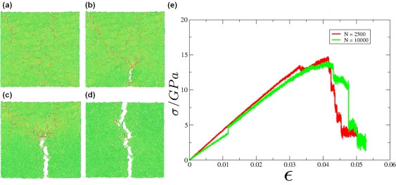
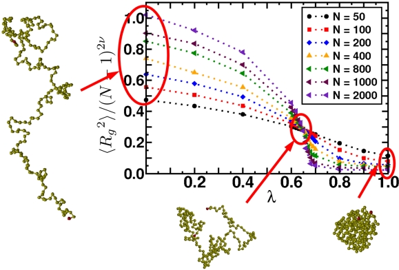
This review discusses several computational methods used on different length and time scales for the simulation of material behavior. First, the importance of physical modeling and its relation to computer simulation on multiscales is discussed. Then, computational methods used on different scales are shortly reviewed, before we focus on the molecular dynamics (MD) method. Here we survey in a tutorial-like fashion some key issues including several MD optimization techniques. Thereafter, computational examples for the capabilities of numerical simulations in materials research are discussed. We focus on recent results of shock wave simulations of a solid which are based on two different modeling approaches and we discuss their respective assets and drawbacks with a view to their application on multiscales. Then, the prospects of computer simulations on the molecular length scale using coarse-grained MD methods are covered by means of examples pertaining to complex topological polymer structures including star-polymers, biomacromolecules such as polyelectrolytes and polymers with intrinsic stiffness. This review ends by highlighting new emerging interdisciplinary applications of computational methods in the field of medical engineering where the application of concepts of polymer physics and of shock waves to biological systems holds a lot of promise for improving medical applications such as extracorporeal shock wave lithotripsy or tumor treatment.

Keywords: biopolymers; computational physics; dendrimers; lithotripsy; modeling and simulation; molecular dynamics; multiscale methods; polymers; shock waves.

Figure 1.

(a) Micrograph section of an etched Al₂O₃ ceramic surface exhibiting the granular structure on the microscale. (b) SEM photograph of the fracture surface of Al₂O₃ after edge-on impact experiment [18] with striking speed of v ≈ 400m/s. (c,d) Microstructural details of the Al₂O₃ surface exhibiting structural hierarchies. Figure by M.O. Steinhauser, Fraunhofer EMI.

Figure 2.

Schematic hierarchical view of structural properties of important classes of materials contrasting typical structural features of inorganic crystalline materials (engineering materials, green) and the structural features of self-organizing organic biological materials (blue). At the nanoscale, the basic constituents of all condensed matter are the atoms bound together in chemical bonds.

Figure 3.

(a) Light microscopic view of a glass fiber reinforced sheet moulding compound (SMC) which is used in car industry as light-weight material. (b) CT-microscopic reconstruction of a section of the laminar glass fiber structure in the material. (c) Scanning Acoustic microscopic view of a tensile-test SMC specimen exhibiting the glass fiber bundles within the compound. Figure by M.O. Steinhauser, Fraunhofer EMI.

Figure 4.

Schematic comparing the relevant length scales in materials science according to [3]. In the field of nano- and microtechnology one usually tries to approach the molecular level from larger scales, miniaturizing technical devices, whereas nature itself always seems to follow a bottom-up approach, assembling and self-organizing its complex (soft) structures from the atomic scale to complex cellular organisms. The typical scopes of important experimental methods using microscopes is displayed as well. The validity of classical physics is limited to length scales down to approximately the size of atoms which, in classical numerical schemes, are often treated as point particles or spheres with a certain eigenvolume.

Figure 5.

Physical, mathematical and numerical modeling scheme illustrated as flow chart. Starting from the experimental evidence one constructs physical theories for which a mathematical formulation usually leads to differential equations, integral equations, or master (rate) equations for the dynamic (i.e., time dependent) development of certain state variables within the system’s abstract state space. Analytic solutions of these equations are very rarely possible, except when introducing simplifications usually involving symmetries. Thus, efficient algorithms for the treated problem have to be found and implemented as a computer program. Execution of the code yields approximate numerical solutions to the mathematical model which describes the dynamics of the physical “real” system. Comparison of the obtained numerical results with experimental data allows for a validation of the used model and subsequent iterative improvement of the model and of theory.

Figure 6.

Principal design of a computer simulation. Usually, some pre-processing as preparation for the main simulation is done with a pre-processor. This piece of computer code might be integrated in the main source code or – in particular in commercial codes –is written as an extra piece of code, compiled and run separately from the main simulation code. During pre-processing, many administration tasks can be done which are not related to the actual simulation run. In large-scale simulations, data are stored during execution for later analysis. This analysis and visualization is done during post-processing. The advantage of separating pre- and post-processing from the actual simulation code is that the code design remains clearly arranged and the important issue of optimization for speed only has to be done for the relevant pieces of the main simulation code. However, in large-scale simulations, involving billions of particles, even the task of data analysis can become a major problem that needs optimization and fast parallelized algorithms [41].

Figure 7.

Design schematic of the particle-based multiscale simulation package “MD-Cube” at EMI. A kernel takes care of administrative tasks. Force modules can be added via defined interfaces as well as modules for the demands of different physical applications.

Figure 8.

(a) The ENIAC (Electronic Numerical Integrator And Computer), one of the first electronic computers that started to operate in 1946. (The very first working electronic computer was the Z3 developed by Konrad Zuse in the 1930s in Germany). The ENIAC weight 30 tons used more than 18.000 vacuum tubes that can be seen in the picture and had a basic clock speed of 10⁵ cycles per second. It was programmed by plugging cables and wires and setting switches using a huge plugboard that was distributed over the entire machine. US Army Photo. (b) Illustration of the available system size (edge length of a simulated cube of classical particles or atoms) and the necessary computer hardware for modern large-scale MD.

Figure 9.

Graph of the total unbounded potential of Equation (25) which allows for modeling the effects of different solvent qualities.

Figure 10.

Illustration of the potential parameters used for modeling bonded interactions.

Figure 11.

Two-dimensional schematic of periodic boundary conditions. The particle trajectories in the central simulation box are copied in every direction.

Figure 12.

MD Optimization schemes for the search of potentially interacting particles. (a) The least efficient all particle “brute force” approach with run time $\mathcal{O}(N^2)$ (b) The linked-cell algorithm which reduces the search effort to $\mathcal{O}(N)$. (c) The linked-cell algorithm combined with neighbor lists which further reduces the search effort by using a list of potentially interacting neighbor particles which can be used for several timesteps before it has to be updated. In this 2D representation, the radius of the larger circle is r_cut + r_skin and the inner circle, which contains actually interacting particles, has radius r_cut.

Figure 13.

Schematic of the sequential construction of different ghost cell layers. An individual cell of the simulation box can be identified by the three integers (i_x, i_y, i_z). The original box in this example has n_x = n_z = 5 and n_y = 4 cells in each direction, i.e., there is no need for the simulation box to have cubic shape. (a) In a first step, all particles of cells with indices (i_x = 1; i_y = 1, ..., n_y; i_z = 1, ..., n_z) are copied into the first layer of ghostparticles. The second layer of ghostparticles then contains all particles pertaining to cells (i_x = 1, ..., n_x; i_y = 1; i_z = 1, ..., n_z) including the ghostparticles of the ghostcells from the first ghostlayer. Finally, the third layer of ghostcells is constructed by copying the particles of the cells with (i_x = 1, ..., n_x; i_y = 1, ..., n_y; i_z = 1) as indicated in the figure.

Figure 14.

(a) Venn diagram of the class P (efficiently solvable problems), class NP (non-deterministic polynomial, i.e., inefficiently solvable problems), and undecidable problems (orange box) for which no algorithms are known. Today, it is generally assumed that all problems in P are contained in the class NP, cf. Figure 14. So far, no proof that decides whether P = NP or P ≠ NP is known. (b) An inefficient algorithm (dashed line) can – for some small values N up to an input number N₀ – be more efficient than a polynomially bounded algorithm (solid line). (c) A real algorithm (dotted line) will always have a run time behavior somewhat in between the worst-case (dashed line) and best-case (solid line) run time.

Figure 15.

Spallation failure in a semi-infinite aluminium target after impact by a 10mm aluminum sphere at 7km/s. (a) Target after impact experiment cut into half. (b) Hydrocode simulation of the impact and related shock propagation leading to the formation of spallation planes.

Figure 16.

(a) Micrograph of a HPC (Al₂O₃) exhibiting the micro structure with an average grain size of 0.7 μm. (b) 2D FEM simulation of a primitive model of this micro structure with a shock impulse traveling through the material from left to right. The plane of the micrograph has been sectioned into 601 × 442 equal-spaced squares which are used as finite elements. The nodes of the upper and lower edge have been assigned $\overrightarrow{\upsilon }=0$ as boundary condition, whereas the leftmost element nodes of the sample are given an initial speed of v_x = 500 m/s. The color code exhibits the pressure profile.

Figure 17.

(a) Voronoi diagram of N=20 sites. For a finite set of generator points $\mathbb{\text{T}}$ ⊂ ${\mathbb{\text{T}}}^d$ the Voronoi diagram maps each p ∈ $\mathbb{\text{T}}$ onto its Voronoi region R(p) consisting of all x ∈ ${\mathbb{\text{T}}}^d$ that are closer to p than to any other point in $\mathbb{\text{T}}$. (b) Delaunay triangulation for the sites in (a).

Figure 18.

5 different Al₂O₃ micrographs (a) and their corresponding grain statistics with respect to the grains’ perimeter (b). The right picture at the bottom of (a) and (b) exhibits a corresponding 2D virtual cut through the 3D PD, i.e., a Voronoi diagram, and its corresponding histogram. Clearly, the histograms both show no Gaussian distribution as was claimed, e.g., by Zhang et al. [167].

Figure 19.

Optimization scheme as suggested in [168]. (a) 2D experimental photomicrograph (top) and an SEM picture of the 3D crystalline surface structure of Al₂O₃ (bottom). (b) 2D virtual slice of a power diagram (top) and the corresponding 3D surface structure obtained from this model. (c) Comparison between 2D experimental data of (a) and the 3D model of (b).

Figure 20.

(a) Area (top) and perimeter (bottom) distribution of one of the Al₂O₃ micrographs of Figure 18 before (black) and after (red) optimization. The bar graphs show the respective histograms of experimental data. (b) Time development of the figure of merit m during the optimization for the structure of (a). After 358000 and 512000 optimization steps, the maximum step size of the reverse MC algorithm (changing the position of a generator point) was increased, which shows a direct influence on the speed of optimization. After 1.5 million steps the deviation between the model and experiment has dropped below 1.3 × 10⁻⁴. The inset shows the corresponding time development of m of the perimeter (red) and (area) distribution of the third central moment.

Figure 21.

3D structures of a meshed PD. In (a) the granular surface structure, its mesh and a detailed augmented section of the mesh at the surface are displayed. (b) A different realization of a 3D structure displaying the possibility of either leaving a (more realistic) rough surface micro structure, or smoothing the surface and thus obtaining a model body with even surface [168].

Figure 22.

Illustration of the multiscale problem. With concurrent FEM methods which include micro structural details, only a very small part of a real system can actually be simulated due to the necessary large number of elements. Figure taken from [172].

Figure 23.

Snapshots of simulations of the edge-on impact system of Figure 22 using a primitive discretization of the geometry of the system in terms of hexahedral elements. (a) FEM with mesh resolution of 0.5mm. (b) FEM with mesh resolution of 1.0mm. (c) SPH with mesh resolution of 0.5mm. All computational results are obtained using a commercial code (Autodyn-3D) and are different in terms of the damage pattern of the cracks propagating through the material 3 μs after impact.

Figure 24.

(a) Schematic of a crystal placed under shock loading. Initially it will compress uniaxially and then relax plastically through defects on the nanoscale, a process known as the one-dimensional to three-dimensional transition. The material may also undergo a structural transformation, represented here as a cubic to hexagonal change. The transformation occurs over a characteristic time scale. The new phase may be polycrystalline solid or melt. Once pressure is released, the microvoids that formed may grow, leading to macroscopic damage that causes the solid to fail. (b) This micrograph shows the voids that occur when a polycrystalline aluminium alloy is shocked and recovered. As the shock wave releases, the voids grow and may coalesce, resulting in material failure.

Figure 25.

The particle Model as suggested in [195]. (a) Overlapping particles with radii R₀ and the initial (randomly generated) degree of overlap indicated by d₀^ij. Here, only two particles are displayed. In the model the number of overlapping particles is unlimited and each individual particle pair contributes to the overall pressure and tensile strength of the solid. (b) Sample initial configuration of overlapping particles (N = 2500) with the color code displaying the coordination number: red (8), yellow (6), and green (4). (c) The same system displayed as an unordered network.

Figure 26.

(a) Schematic of the intrinsic scaling property of the proposed material model. Here, only the 2D case is shown for simplicity. The original system (Model M_a) with edge length L₀ and particle radii R₀ is downscaled by a factor of 1/a into the subsystem Q_A of M_A (shaded area) with edge length L, while the particle radii are upscaled by factor a. As a result, model M_B of size aL = L₀ is obtained containing much fewer particles, but representing the same macroscopic solid, since the stress-strain relation (and hence, Young’s modulus E) upon uni-axial tensile load is the same in both models. (b) Young’s modulus E of systems with different number of particles N in a stress-strain (σ–ε) diagram. In essence, E is indeed independent of N.

Figure 27.

Sample configurations of systems with N = 10000 particles and different particle densities Ω. The color code displays the coordination numbers: blue (0), green (4), yellow (6), red (8). (a) Ω = 0.7. (b) Ω = 0.9 (c) Ω = 1.3 (d) Ω = 1.7 (e) Breaking strength σ_b for different system sizes N (filled symbols) as a function of particle density Ω, compared with the theoretical breaking strength σ_max (open symbols). The inset shows the stress-strain (σ – ε) relation for systems with three different initial expansion times τ. In essence, the larger the expansion time for the generation of the random initial overlap of particles, the larger is the material strength σ_max.

Figure 28.

Crack initiation and propagation in the virtual macroscopic material sample upon uni-axial tensile load using N = 10⁴ particles. The color code is: Force-free bonds (green); Bonds under tensile load (red). (a) Initiation of local tensions. (b) Initiation of a crack tip with local tensions concentrated around this crack tip. (c) Crack propagation including crack instability. (d) Failure. (e) Averaged stress-strain (σ-ε) relation. For N = 2500 (green curve) 10 different systems were averaged, and for N = 10000 (red curve) the stress-strain relations of 5 different initial particle configurations obtained in uni-axial load simulations were averaged.

Figure 29.

Snapshots of a 2D FEM simulation of the fracture process of a PMMA (poly-methyl methacrylate) plate which is subject to an initial uniform strain rate in vertical direction. Here, there is no statistical variability of the microstructure modeled with more than 50 × 10⁶ elements. Thus, the model solid has to be artificially pre-notched and it still exhibits a strong dependence on the mesh size and the number of elements. Adapted from [202].

Figure 30.

Quasi-static shear loading of a virtual material specimen with N = 2500. The color code is the same as in Figure 28 except for particle bonds under pressure which are coded in blue. (a) Onset of shear tensile bands and (orthogonal) shear pressure bands in the corners of the specimen. (b) Shear bands traversing the whole specimen. (c) Ultimate failure.

Figure 31.

Results of a simulation of the edge-on-impact (EOI) geometry, cf. Figure 23, except this time, the whole macroscopic geometry of the experiment can be simulated while still including a microscopic resolution of the system. The impactor is not modeled explicitly, but rather its energy is transformed into kinetic energy of the particle bonds at the impact site. (a) Top row: A pressure wave propagates through the material and is reflected at the free end as a tensile wave (not shown). Middle row: The actual EOI experiment with a SiC specimen. The time interval between the high-speed photographs is comparable with the simulation snapshots above. The red arrows indicate the propagating shock wave front. Bottom row: The same simulation run but this time only the occurring damage in the material with respect to the number of broken bonds is shown. (b) Number of broken bonds displayed for different system sizes N, showing the convergence of the numerical scheme. Simulation parameters (α, γ, λ) are chosen such that the correct stress-strain relations of two different materials (Al₂O₃ and SiC) are recovered in the simulation of uniaxial tensile load. The insets show high-speed photographs of SiC and Al₂O₃, respectively, 4 μs after impact.

Figure 32.

A coarse-grained model of a polymer chain where some groups of the detailed atomic structure (yellow beads) is lumped into one coarse-grained particle (red). The individual particles are connected by springs (bead-spring model).

Figure 33.

General set up of a scattering experiment according to [206]. Details are described in the main text.

Figure 34.

Coil-to-globule transition from good to bad solvent behavior of a polymer chain. Plot of 〈R_g²〉 / (N – 1)^2ν vs. interaction parameter λ for linear chains. The points represent the simulated data and the dotted lines are guides to the eye. ν = ν_θ = 0.5. Also displayed are simulation snapshots of linear chains for the three cases of a good, θ-, and a bad solvent.

Figure 35.

Interaction parameter λ of Equation (25) vs. N^−1/2 for different values of the scaling function. Data points are based on the radius of gyration of linear chains [51].

Figure 36.

Kratky plot of S(q) of linear chains (N = 2000) for different values of the interaction parameter λ.

Figure 37.

(a) Log-Log plot of 〈R_g²〉 vs. N of star polymers with different arm numbers f. For comparison, data for linear chains (f = 2) are displayed as well. (b) Scaling plot of the corrections to scaling of 〈R_g²〉 (f) plotted vs. N⁻¹ in good solvent. For clarity, the smallest data point of the linear chains (f = 2, N = 50) is not displayed.

Figure 38.

(a) S(q) of single linear chains with N = 700 and varying stiffness k_θ. The scaling regimes (fully flexible and stiff rod) are indicated by a straight and dashed line, respectively. (b) Scaling plot of S(q)/l_K versus q · l_K using the statistical segment length l_K adapted from [208].

Figure 39.

Simulation snapshots of (a) flexible chains (k_θ = 0), (b) semiflexible chains (k_θ = 20), (c) stiff, rod-like chains (k_θ = 50).

Figure 40.

Twisted, DNA-like polyelectrolyte complexes formed by electrostatic attraction of two oppositely charged linear macromolecules with N = 40 at τ̂ = 0 (a), τ̂ = 10500 (b), τ̂ = 60000 (c) and τ̂ = 120000 (d), where τ̂ is given in Lennard-Jones units. The interaction strength is ξ = 8 [222,223].

Figure 41.

(a) Radii of gyration as a function of the interaction strength ξ for various chain lengths according to [223]. The radius of gyration R_g² is scaled by (N – 1)^2/3, where (N –1) is the number of bonds of a single chain. Also displayed are sample snapshots of the collapsed globules with N = 40 and interaction strengths ξ = 0.4, 4, 40. (b) Radial density of monomers with respect to the center of mass of a globule and interaction strength ξ = 4 for different chain lengths, N = 20 (blue), N = 40 (red), N = 80 (green) and N = 160 (brown).

Figure 42.

(a) Hierarchical features of collagen which determines the mechanical properties of cells, tissues, bones and many other biological systems, from atomistic to microscale. Three polypeptide strands arrange to form a triple helical tropocollagen molecule. Tropocollagen (TP) molecules assemble into collagen fibrils which mineralize by formation of hydroxipatite (HA) crystals in the gap regions which exist due to a staggered array of molecules. (b) Stress-strain response of a mineralized collagen fibril exhibiting larger strength than a non-mineralized, pure collagen fibril. Both figures adapted from [227] with permission.

Figure 43.

(a) Schematic of the principle of ESWL. (b) Image of human body with symptomatic fibroids. Sonication pathway is superimposed on the image and the spot where irreversible thermal damage is expected is also superimposed onto this image. Adapted from [230] with permission. (c) Schematic of a magnetic resonance guided HIFU equipment for the possible treatment of tumor tissue. Figure adapted from [231] with permission.

Figure 44.

Scheme of the disintegration of a kidney stone as a result of direct and indirect shock wave effects. Figure adapted from [235] with permission.

References

1. Phillips R. Crystals, Defects and Microstructures—Modeling Across Scales. Cambridge University Press; Cambridge, UK: 2001.
1. Yip S, editor. Handbook of Materials Modeling. Springer; Berlin, Germany: 2005.
1. Steinhauser MO. Computational Multiscale Modeling of Solids and Fluids—Theory and Applications. Springer; Berlin/Heidelberg/New York, Germany/USA: 2008.
1. Hockney R, Eastwood J. Computer Simulation Using Particles. McGraw-Hill; New York, NY, USA: 1981.
1. Ciccotti G, Frenkel G, McDonald I. Simulation of Liquids and Solids. North-Holland; Amsterdam, The Netherlands: 1987.
Publication types
LinkOut - more resources