Image correlation microscopy for uniform illumination

Abstract

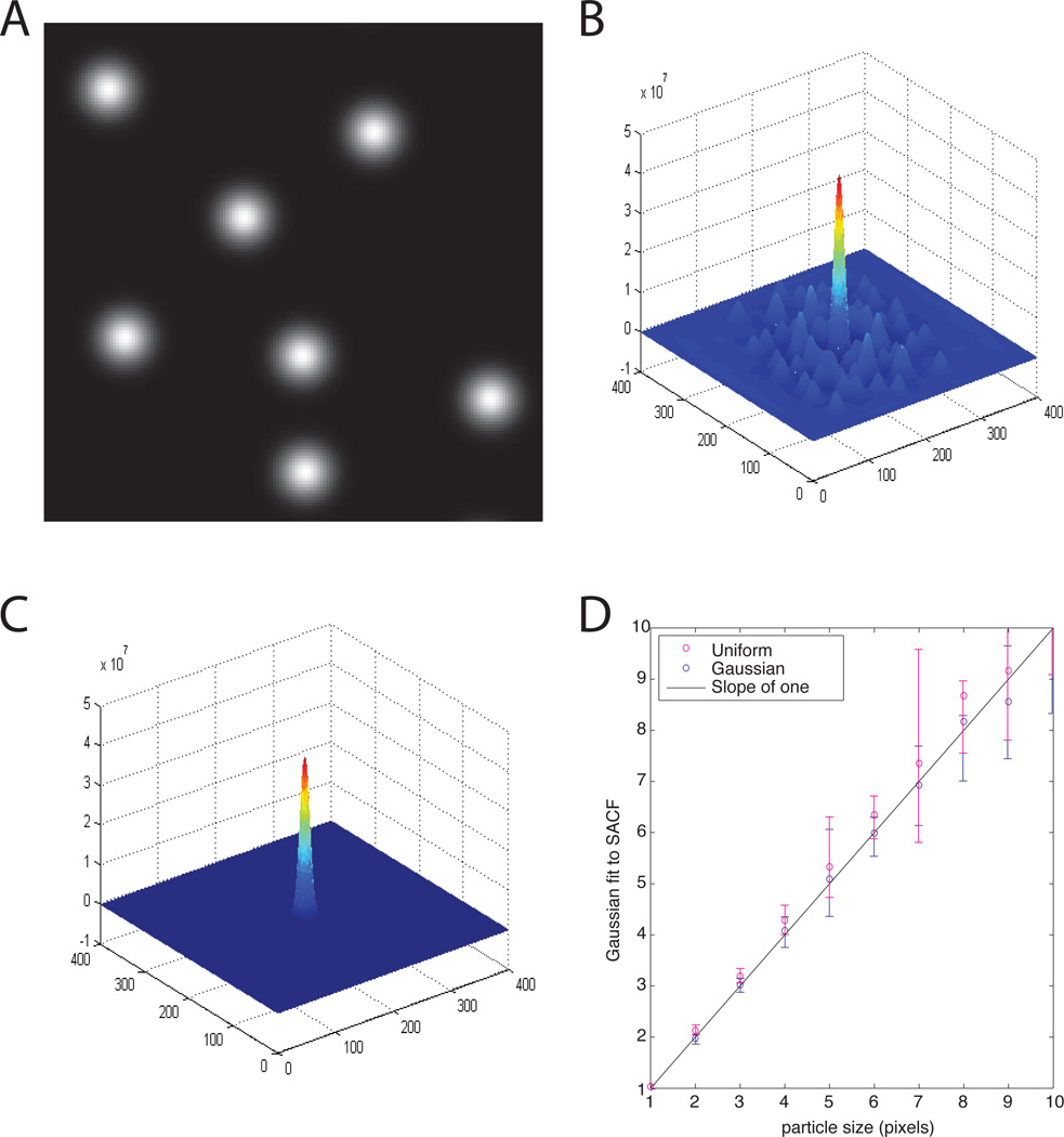
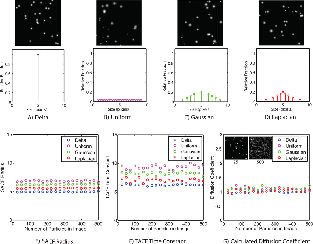
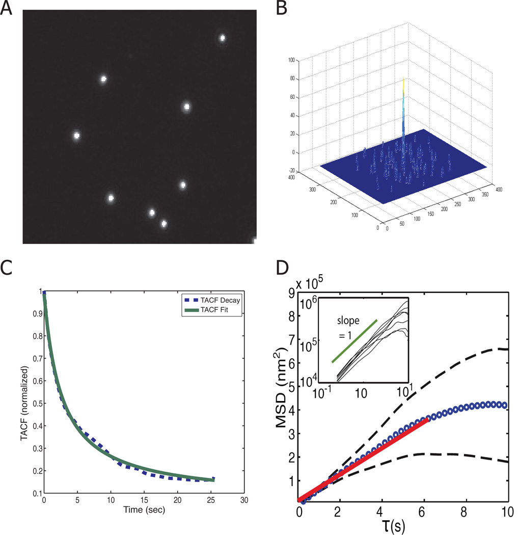
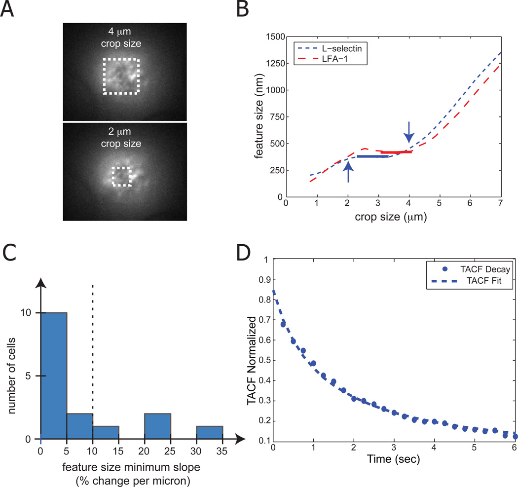
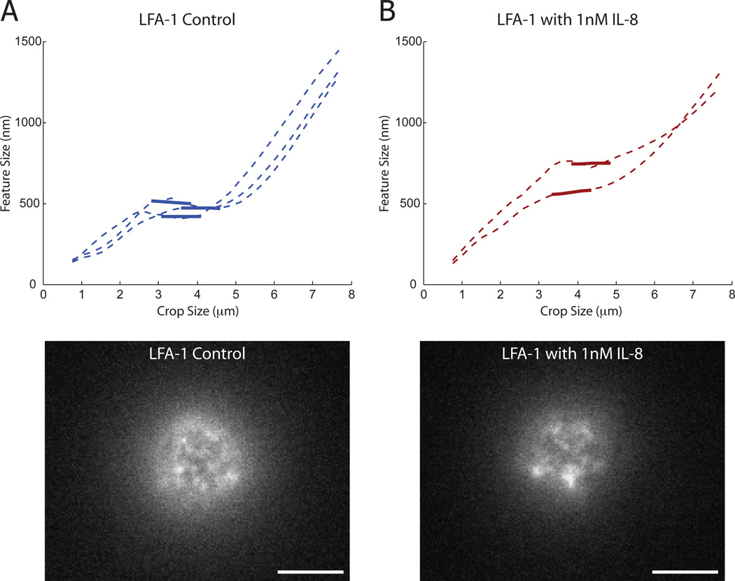
Image cross-correlation microscopy is a technique that quantifies the motion of fluorescent features in an image by measuring the temporal autocorrelation function decay in a time-lapse image sequence. Image cross-correlation microscopy has traditionally employed laser-scanning microscopes because the technique emerged as an extension of laser-based fluorescence correlation spectroscopy. In this work, we show that image correlation can also be used to measure fluorescence dynamics in uniform illumination or wide-field imaging systems and we call our new approach uniform illumination image correlation microscopy. Wide-field microscopy is not only a simpler, less expensive imaging modality, but it offers the capability of greater temporal resolution over laser-scanning systems. In traditional laser-scanning image cross-correlation microscopy, lateral mobility is calculated from the temporal de-correlation of an image, where the characteristic length is the illuminating laser beam width. In wide-field microscopy, the diffusion length is defined by the feature size using the spatial autocorrelation function. Correlation function decay in time occurs as an object diffuses from its original position. We show that theoretical and simulated comparisons between Gaussian and uniform features indicate the temporal autocorrelation function depends strongly on particle size and not particle shape. In this report, we establish the relationships between the spatial autocorrelation function feature size, temporal autocorrelation function characteristic time and the diffusion coefficient for uniform illumination image correlation microscopy using analytical, Monte Carlo and experimental validation with particle tracking algorithms. Additionally, we demonstrate uniform illumination image correlation microscopy analysis of adhesion molecule domain aggregation and diffusion on the surface of human neutrophils.

Figure 1

Decay in the temporal autocorrelation function (TACF) is not significantly impacted by particle shape. (A) The correlation decay for random diffusion of Gaussian intensity particles given by Eq. 6 (solid line) shows strong agreement with the random diffusion of uniform intensity disks given by Eq. 8 (circles). (B) Simulated random diffusion of particles displayed as either Gaussian (left) or uniform (right) intensity. 50 particles with a radius of 10 pixels were seeded over a 200 × 200 image matrix. (C) Correlation decay for simulated diffusing points represented as Gaussian particles (solid line) is very similar to to the same points represented as uniform disks (circles). (D) Diffusion length scales calculated from characteristic correlation decay correspond to the appropriate particle size for both Gaussian and uniform intensity. Three simulations were run for each type of particle at each particle size.

Figure 2

Characteristic diffusion length is calculated from the Spatial Autocorrelation Function (SACF). (A) Gaussian illumination particles are randomly positioned on a 200 × 200 image matrix in MATLAB. (B) SACF is calculated for the simulated particles from (A). (C) Gaussian fit to the SACF. (D) Both simulated Gaussian and uniform intensity particles of various sizes are accurately measured with the Gaussian fit to SACF. Any deviation from the straight line was due to random positioning of particles, in which case some overlapped or were on the edge of the image matrix. Three simulations were run for each type of particle at each pixel size.

Figure 3

Diffusion coefficients can be accurately predicted by UI-ICM even for complex particle size distributions. Diffusion was simulated for all particles as a two-dimensional random walk of one pixel per unit time on a 64 × 64 pixel image matrix. Simulations were run with four different distributions of Gaussian particle sizes, each with a 5 pixel mean radius: (A) Monodisperse particle size, (B) Uniform distribution, (C) Gaussian distribution, and (D) Laplacian distribution. Representative images show 50 particles randomly distributed. (E) SACF was calculated for each distribution with between 25 and 500 Gaussian particles randomly positioned across the image matrix. The maximum density resulted in many overlapping particles. Overlapping particle intensity was additive and was not thresholded; still, increasing the density of particles did not change the SACF radius. Although all distributions had the same mean radius, SACF radius is weighted more heavily by larger particles in the field (F) TACF was calculated for each distribution with between 25 and 500 Gaussian particles. Like the SACF, the TACF time constant was independent of particle density for each distribution, but biased toward larger particles. (G) Diffusion coefficients were calculated for each distribution at varying particle densities based on Eq. 8. The calculated diffusion coefficient for all distributions converged to 1 pixel per unit time for all densities and distributions, matching the simulation input. Insets show representative samples of 25 and 500 Gaussian particles of uniform size distribution.

Figure 4

Fluorescent bead diffusion measurement with UI-ICM and validation with a particle tracking algorithm. 0.93 um fluorescent beads in 1x PBS were assembled into a 10 um thick chamber and observed at room temperature in an inverted fluorescence microscope. Images were taken every 100 ms for 25 seconds. (A) A characteristic static image of fluorescent beads in a 10 µm thick chamber. (B) SACF for the fluorescent beads. (C) TACF is plotted over 25 seconds. The data (blue dashed line) is well fit by Eq. 6 (green solid line). Using the characteristic time from the TACF decay and the size from SACF, the diffusion coefficient is calculated as 1.2 × 10⁻¹⁰ cm²/sec using UI-ICM. (D) The same fluorescent beads were tracked with a particle tracking algorithm and the average mean squared displacement (MSD) for 41 particles in two time-lapse movies are shown in blue circles. Black dashed curves indicate one standard deviation above and below the mean. A linear fit to the early time data shown in bold red yields D = 1.4 × 10⁻¹⁰ cm²/sec. The inset shows a log-log plot of a random sub-sample of the data compared to the ideal diffusive slope of 1.

Figure 5

UI-ICM application to a spherical cell. To analyze receptor domain dynamics on the surface of human neutrophils (8–9 um diameter), it is necessary to analyze only the dynamic region of the image. Cells resting on the coverslip have a ‘footprint’ diameter of approximately 4 um using our non-confocal epi-fluorescence microscope. (A) Gaussian fit to the SACF defines the centroid of the cell. Crop sizes centered around the centroid are varied to determine the ideal region of interest (ROI). Black dash boxes show the size of a 2 and 4 um crop size (B) Feature size extraction from the SACF for two cells labeled for L-selectin or LFA-1 adhesion molecules is dependent on the crop size. Feature sizes from small crop sizes (< 2 um) are primarily a function of noise in the image. In most cells, there is a plateau region (2–4 um) where the feature size in not dependent on crop size. At larger crop sizes (> 4 um), the cell itself is the primary feature and significantly affects feature size extraction. For each cell, the minimum slope (thick line) over a one micron crop size is found. The mean SACF width in this region is used to determine the feature size. (C) Histogram of minimum slopes. Cells that do not have a plateau with a minimum slope less than 10% are not further analyzed. (D) The TACF for a representative neutrophil is measured over six seconds. The data (circles) is well fit by Eq. 6 (dashed line).

Figure 6

Adhesion molecule cluster formation upon neutrophil stimulation with IL-8. Human neutrophils were labeled for LFA-1 with fluorescent monoclonal antibody. (A) Control cells had a feature size of 490 nm using the method described in Figure 5. Three plots are shown. A characteristic image of an untreated cell is shown below. (B) Cells were then activated with 1 nM IL-8 for 15 minutes and imaged. Two cells that maintained a spherical morphology where analyzed. The feature size increased to 640 nm. A characteristic image shows a clear increase in receptor domain size. White scale bar is 5 microns.

References

1. Bates IR, Wiseman PW, Hanrahan JW. Investigating membrane protein dynamics in living cells. Biochem Cell Biol. 2006;84:825–831. - PubMed
1. Cairo CW, Mirchev R, Golan DE. Cytoskeletal regulation couples LFA-1 conformational changes to receptor lateral mobility and clustering. Immunity. 2006;25:297–308. - PubMed
1. Cheezum MK, Walker WF, Guilford WH. Quantitative comparison of algorithms for tracking single fluorescent particles. Biophys J. 2001;81:2378–2388. - PMC - PubMed
1. Digman MA, Brown CM, Horwitz AR, Mantulin WW, Gratton E. Paxillin dynamics measured during adhesion assembly and disassembly by correlation spectroscopy. Biophys J. 2008;94:2819–2831. - PMC - PubMed
1. Ehrenberg M, McGrath JL. Binding between particles and proteins in extracts: implications for microrheology and toxicity. Acta Biomater. 2005;1:305–315. - PubMed