. 2010 Jan 13;30(2):767-84.
doi: 10.1523/JNEUROSCI.4170-09.2010.

Temporal codes for amplitude contrast in auditory cortex

Affiliations

Temporal codes for amplitude contrast in auditory cortex

Brian J Malone et al. J Neurosci. .

Abstract

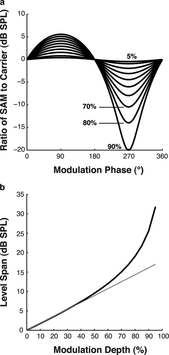
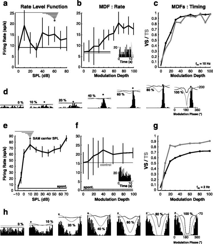
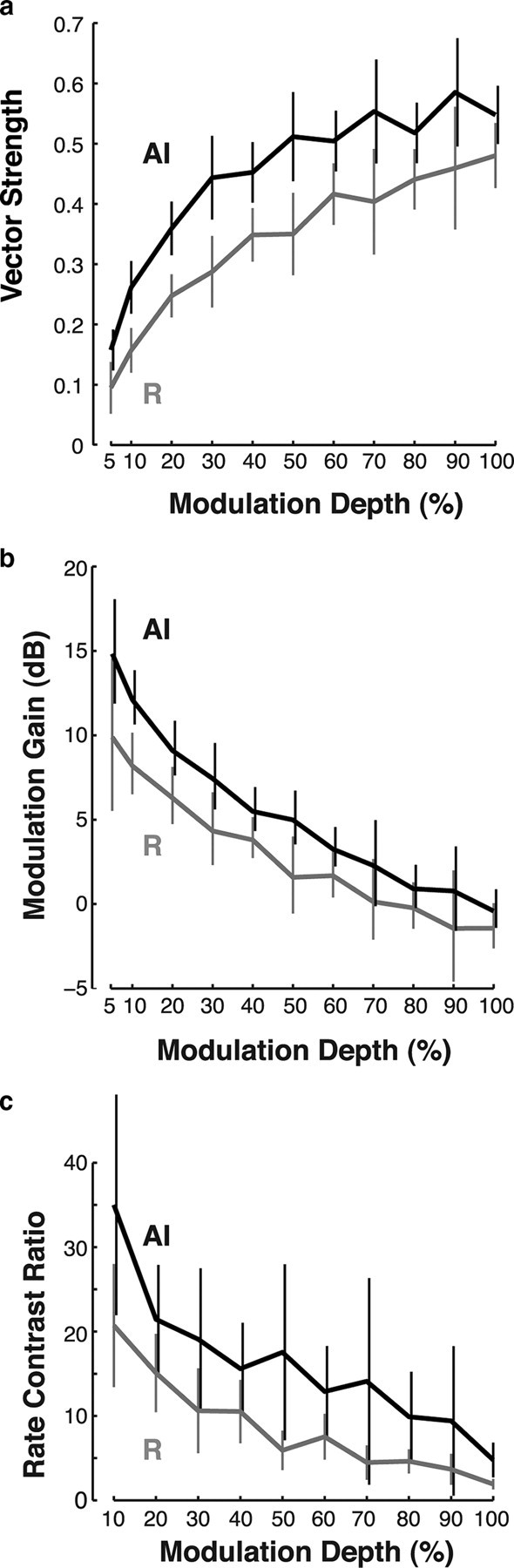
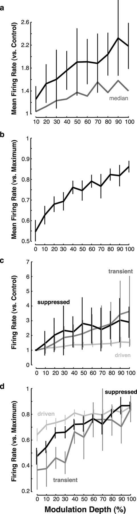
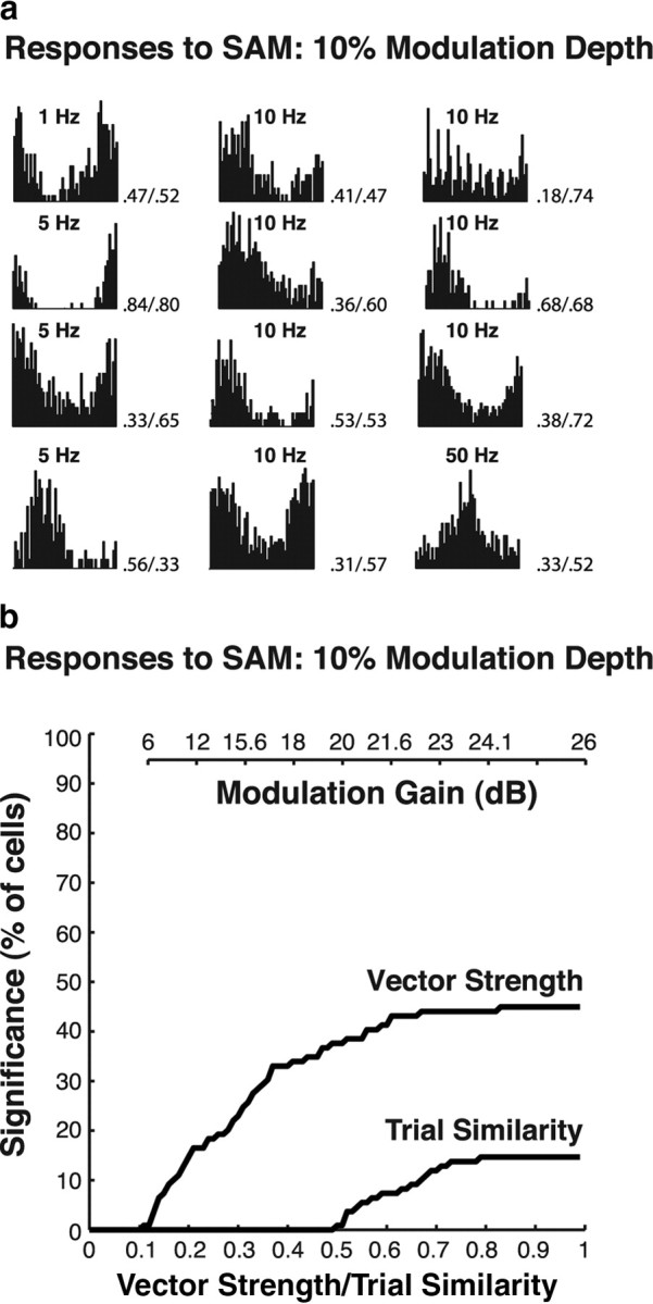
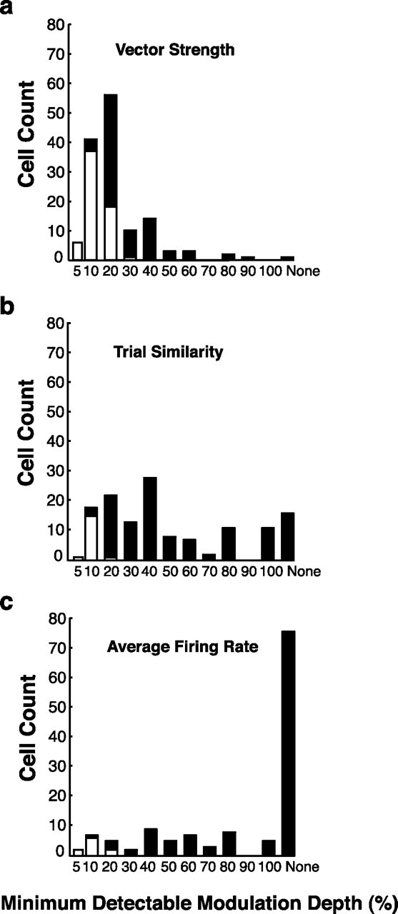
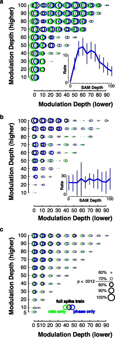
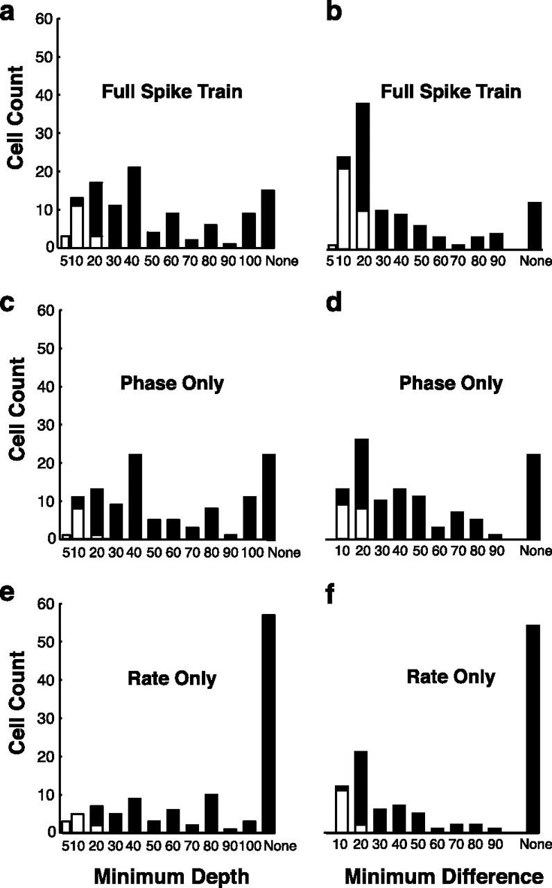
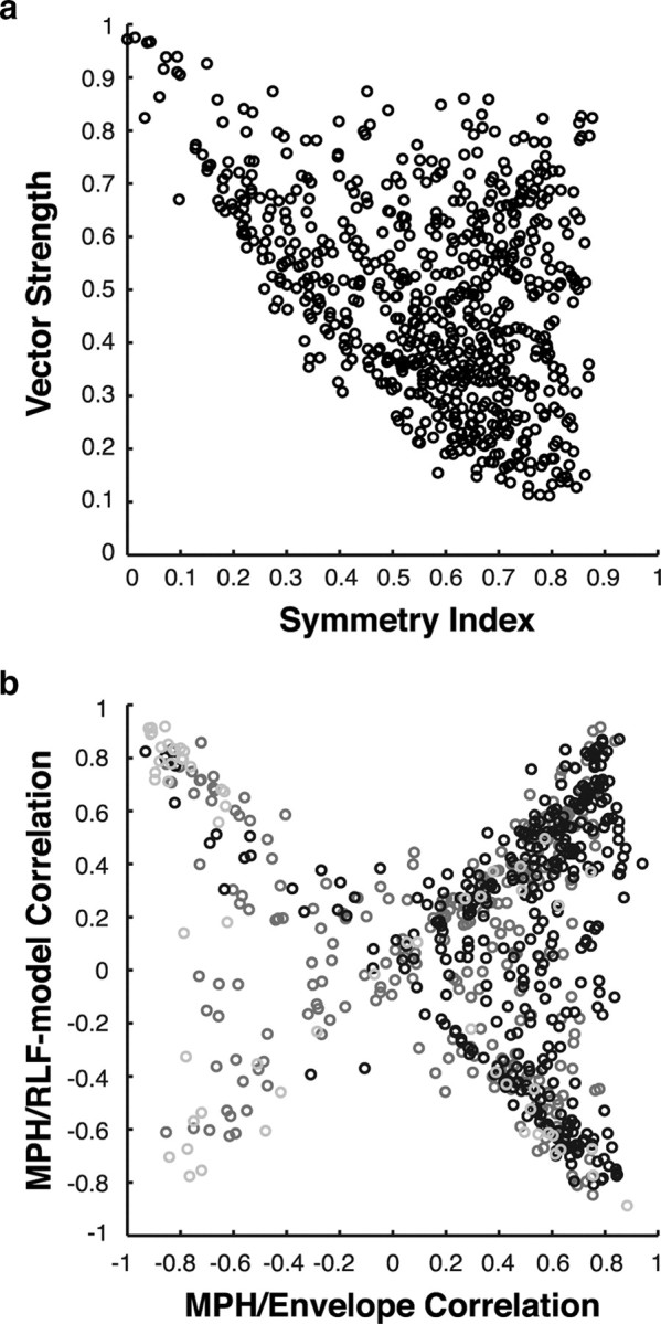
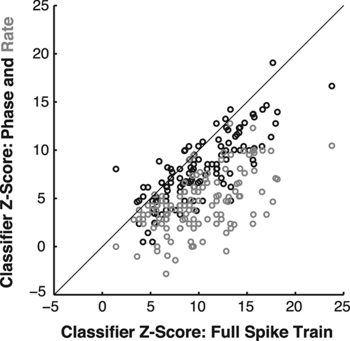
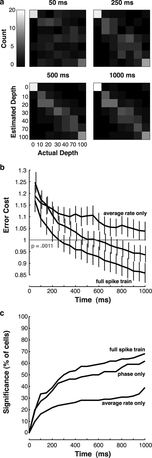
The encoding of sound level is fundamental to auditory signal processing, and the temporal information present in amplitude modulation is crucial to the complex signals used for communication sounds, including human speech. The modulation transfer function, which measures the minimum detectable modulation depth across modulation frequency, has been shown to predict speech intelligibility performance in a range of adverse listening conditions and hearing impairments, and even for users of cochlear implants. We presented sinusoidal amplitude modulation (SAM) tones of varying modulation depths to awake macaque monkeys while measuring the responses of neurons in the auditory core. Using spike train classification methods, we found that thresholds for modulation depth detection and discrimination in the most sensitive units are comparable to psychophysical thresholds when precise temporal discharge patterns rather than average firing rates are considered. Moreover, spike timing information was also superior to average rate information when discriminating static pure tones varying in level but with similar envelopes. The limited utility of average firing rate information in many units also limited the utility of standard measures of sound level tuning, such as the rate level function (RLF), in predicting cortical responses to dynamic signals like SAM. Response modulation typically exceeded that predicted by the slope of the RLF by large factors. The decoupling of the cortical encoding of SAM and static tones indicates that enhancing the representation of acoustic contrast is a cardinal feature of the ascending auditory pathway.


Figures

Figure 1.
Figure 1.
On a decibel axis, larger modulation depths produce larger decreases than increases in SPL and span much greater ranges. a, Changes in the instantaneous SPL, in decibels, of the SAM stimulus relative to an unmodulated stimulus at the same carrier level. The curves represent modulation depths ranging from 10 to 90% in 10% steps, as well as the lowest depth tested, 5%. The instantaneous SPL achieves its minimum at 270° because all modulations were presented in sine phase. b, Span, in dB SPL, of the modulation as a function of modulation depth. The level span is defined as the difference between the maximum and minimum instantaneous SPL (in decibels) within each modulation cycle. The gray line indicates the result if the level span increased linearly with modulation depth, which it nearly does up to values of 40%.
Figure 2.
Figure 2.
Cortical encoding of sound level varies substantially from neuron to neuron. a–h, Shown here are the responses from two cells in auditory cortex (a–d and e–h). a, d, Rate level functions obtained for each of these cells. On all panels, vertical lines indicate ±2 SEM of measurement. Circles on a point of the RLF indicate that the firing rate was elevated relative to the spontaneous rate (Wilcoxon rank-sum; p < 0.001). The small circular icon indicates the carrier level used to obtain the rate modulation depth functions depicted in b and f. The series of small horizontal lines above the carrier level icons (a, e) illustrates the level span of the SAM stimuli comprising the MDF. The larger horizontal line indicates the spontaneous firing rate averaged over the interstimulus intervals. This convention is maintained in b and f. The additional horizontal gray line indicates the response to the unmodulated control stimulus, which is also shown in PSTH form as an inset (gray bars in the insets represent spikes during the interstimulus interval). c, g, Vector strength (black) and trial similarity (gray) obtained across modulation depth. Filled circles on the VS and TS curves indicate significance at the p < 0.001 level (VS: Rayleigh test >13.816; TS: bootstrap; see Materials and Methods). The inset text indicates the modulation frequency. d, h, MPHs elicited by the modulation depths indicated on each panel. All MPHs have been rotated (90°) so that the instantaneous minimum SPL of the SAM stimulus is centered in the panel. The small circles indicate the mean phase of the response. The gray curves above each panel indicate the change in instantaneous SPL (Fig. 1a). The black curves indicate the modulation in firing rate predicted by the instantaneous SPL and the RLF. These curves are intended to indicate relative modulation, rather than absolute spike rates, and are vertically placed so their maximum aligns with the maximum spike counts in a single bin of the MPH. These curves have been rotated by the average minimum latency for each neuron.
Figure 3.
Figure 3.
Cortical responses provide high-contrast representations of shallow modulation depths. a, Plot of the population average of vector strength against the modulation depth. b, Plot of the population average of modulation gain in decibels (see Materials and Methods) against the modulation depth. c, Plot of the rate contrast ratio (see Materials and Methods) against the modulation depth. On all curves, vertical lines indicate ±2 SEM, black curves represent data from AI, and gray curves represent data from R.
Figure 4.
Figure 4.
Firing rates averaged across the population increase with modulation depth to a degree predicted by the response to the unmodulated control tone. a, How the population average (black curve) firing rate varies across modulation depth when normalized by the firing rate elicited by an unmodulated control tone at the same carrier level and frequency. The gray curve shows the changes in the median firing rate. In all panels, vertical lines indicate ±2 SEs of measurement. b, Same data normalized by the maximum firing rate achieved within the MDF. c, d, Similar to a and b, respectively, but the data have been subdivided by the MTF-derived response class, so the light gray curve represents the driven response class, the dark gray curve the transient class, and the back curve the suppressed class (see Materials and Methods). Vertical lines indicate ±2 SEM.
Figure 5.
Figure 5.
Shallow (10%) modulations of amplitude produce robust cycle-by-cycle response modulation in the most sensitive cortical neurons. a, MPHs obtained for 10% SAM for 12 neurons. With the exception of the neuron in the top right panel, the responses of these cells produced the highest values of the Rayleigh statistic in the sample and thus represent the upper limit of modulation sensitivity we encountered. The modulation frequency used is indicated in bold, and the VS/TS values are shown to the right of each MPH. The MPH at the top right is modulated at both the modulation frequency (10 Hz) and the carrier (100 Hz). b, Population distribution (n = 109) of vector strength and trial similarity for 10% SAM as cumulative distribution curves. Note that the relative displacement of the two curves reflects different significance criteria (see Materials and Methods). For convenience, the modulation gain (decibel) equivalent to each of the VS labels is shown above.
Figure 6.
Figure 6.
Measures of temporal structure in the MPH predict lower modulation detection thresholds than measures of average firing rate. a–c, Histograms indicate the lowest modulation depth that produced a significant VS (a), significant TS (b), or significant change in firing rate relative to the unmodulated control (c). White bars indicate that the result was obtained at the lowest modulation depth presented to the cell, allowing for the possibility that the actual threshold is lower. Black bars indicate that the threshold value obtained was not the lowest tested modulation depth. The designation “None” means that a threshold value was not obtained for any tested depth.
Figure 7.
Figure 7.
Classifier performance for pairwise discrimination of SAM stimuli varying in modulation depth illustrates how both spike timing and spike rate information contribute to modulation depth discrimination. The modulation depth for the first stimulus in the pair is mapped to the abscissa, and the depth for the second is mapped to the ordinate. Differences in modulation depth vary with the distance from the diagonal. The performance of the classifiers, in percentage correct, is indicated by the diameter of each circle, such that 50% = 0. The icons in the bottom right panel indicate how performance relates to circle size. Performance that is significantly above chance is indicated by heavier line weighting (72.5% corresponds to a p value of ∼0.001). Black circles represent the performance of the full spike train classifier; blue circles: the phase-only classifier; green circles: the rate-only classifier. a, b, Results for individual neurons. The insets show the RLFs for each neuron (vertical lines indicate ±2 SEM). c, Classifier performance for each comparison averaged over the population.
Figure 8.
Figure 8.
Distributions of minimum detectable modulation depths and differences obtained with spike train classification techniques indicate that spike timing information is crucial for many cells. a, c, e, Left histograms indicate the lowest modulation depth that could be reliably (72.5% corresponds to a p value of < 0.001) discriminated from the unmodulated control tone. b, d, f, Right histograms indicate the smallest difference in modulation depth (e.g., for 10%, 10 vs 20%, or 50 vs 60%) that could be reliably discriminated by the classifiers. The classifier type is indicated above each panel. White bars indicate that the result was obtained at the lowest modulation depth (a, c, e) or modulation depth difference (b, d, f) presented to the cell, allowing for the possibility that the actual threshold is lower. Black bars indicate that the threshold value obtained was not the lowest tested modulation depth.
Figure 9.
Figure 9.
Analysis of MPH symmetry and the similarity of MPH shape to SAM envelopes indicates a dissimilarity in the encoding of static and dynamic level differences. a, Distribution of SIs, which quantify the mirror symmetry of the response (the envelope of SAM is mirror symmetric) as a function of VS. b, Scatterplot comparing the correlations between MPH shapes and the SAM envelope profiles (in decibels; abscissa) against the correlations between the MPH shapes and the MPHs predicted on the basis of the RLF (see Materials and Methods). Black circles indicate the responses of neurons with driven responses to the unmodulated control tone, dark gray circles indicate transient responses, and light gray circles indicate suppressed responses. In both panels, the data represent all tested neurons at all tested modulation depths, so a single neuron may contribute as many points to the graph as there were points in its MDF that elicited significant modulation.
Figure 10.
Figure 10.
Temporal discharge patterns reliably discriminate tone pip stimuli varying in SPL. Results from the phase-only (black) and rate-only (gray) classifiers are plotted against classifier performance for the full spike train. The diagonal line indicates performance equal to that of the full spike train classifier.
Figure 11.
Figure 11.
Classifier performance varies with the analysis epoch duration. a, Four confusion matrices obtained at varying epoch durations (50, 250, 500, and 1000 ms). Correct identification of the SAM stimuli is indicated by the number of entries along the diagonal of the matrix. Each stimulus was subdivided into 20 epochs, so each cell of the matrix can vary from 0 to 20. The error costs for these four confusion matrices were 0.92, 0.47, 0.40, and 0.39 for 50, 250, 500, and 1000 ms, respectively. b, How the population average of the error cost varies as a function of the epoch duration for each of the classifiers. Error cost for each neuron was normalized relative to the error cost that would be significant at the criterion level (p < 0.0012) for a confusion matrix of the equivalent size. c, Set of cumulative distribution curves indicating the percentage of cells that achieved better-than-chance classifier performance in terms of error cost (p < 0.0012) as a function of the analysis epoch duration.

Similar articles

Cited by

References

    1. Bieser A, Müller-Preuss P. Auditory responsive cortex in the squirrel monkey: neural responses to amplitude-modulated sounds. Exp Brain Res. 1996;108:273–284. - PubMed
    1. Billimoria CP, Kraus BJ, Narayan R, Maddox RK, Sen K. Invariance and sensitivity to intensity in neural discrimination of natural sounds. J Neurosci. 2008;28:6304–6308. - PMC - PubMed
    1. Busby PA, Tong YC, Clark GM. The perception of temporal modulations by cochlear implant patients. J Acoust Soc Am. 1993;94:124–131. - PubMed
    1. Cazals Y, Pelizzone M, Saudan O, Boex C. Low-pass filtering in amplitude modulation detection associated with vowel and consonant identification in subjects with cochlear implants. J Acoust Soc Am. 1994;96:2048–2054. - PubMed
    1. Cohen YE, Theunissen F, Russ BE, Gill P. Acoustic features of rhesus vocalizations and their representation in the ventrolateral prefrontal cortex. J Neurophysiol. 2007;97:1470–1484. - PubMed

Publication types

LinkOut - more resources