Linear and nonlinear relationships between visual stimuli, EEG and BOLD fMRI signals

Abstract

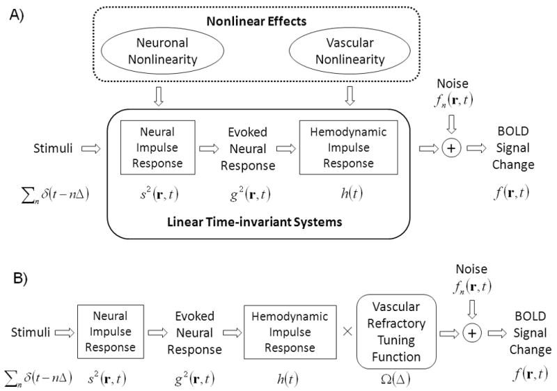
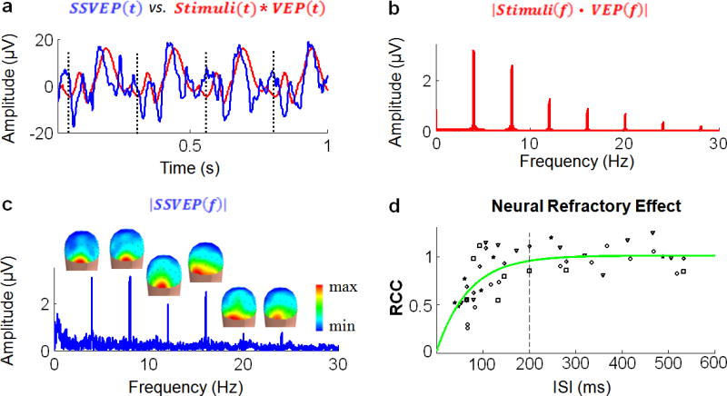
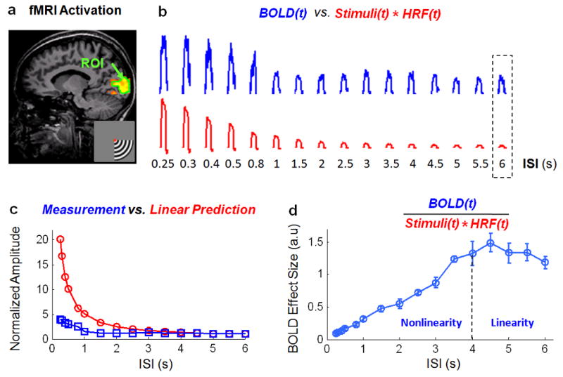
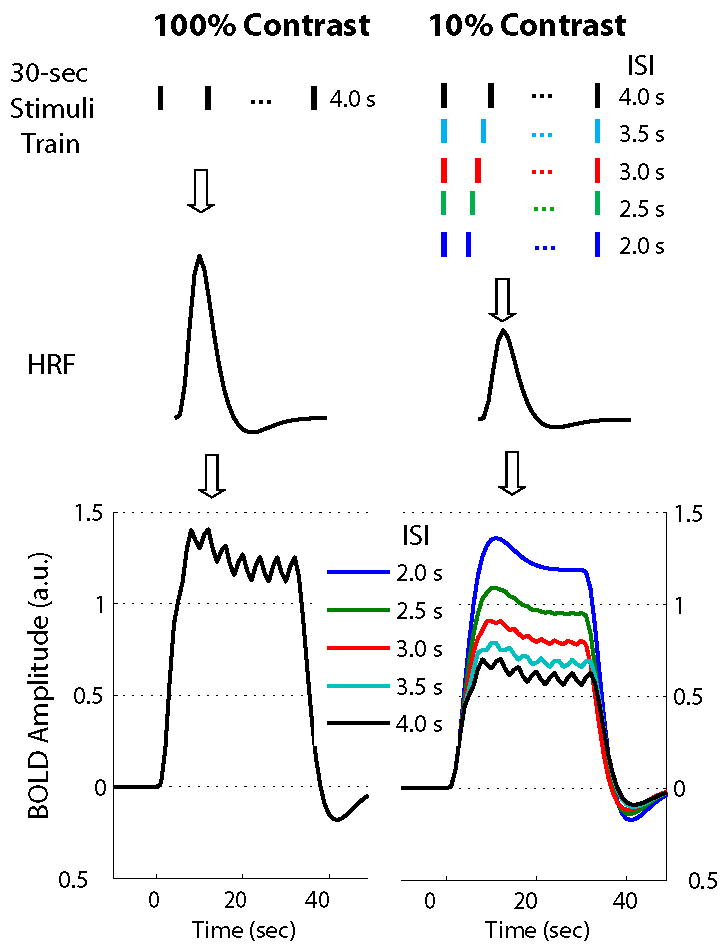
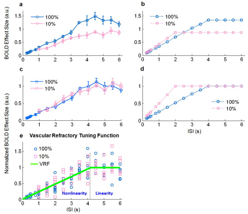
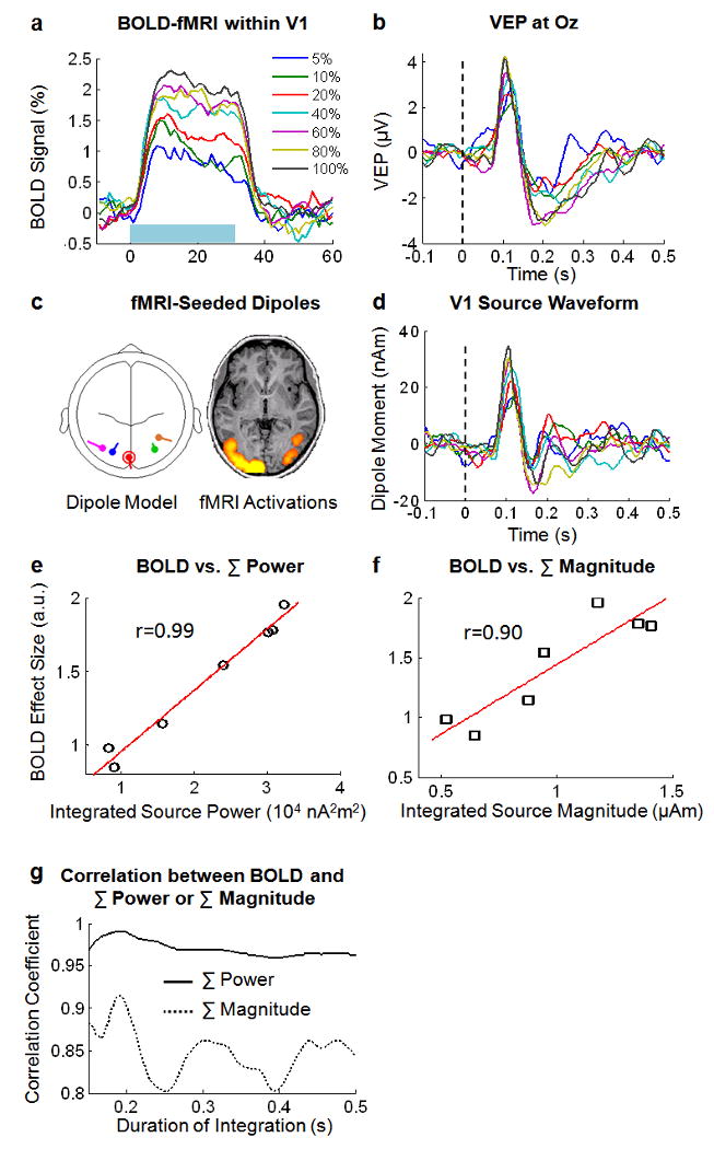
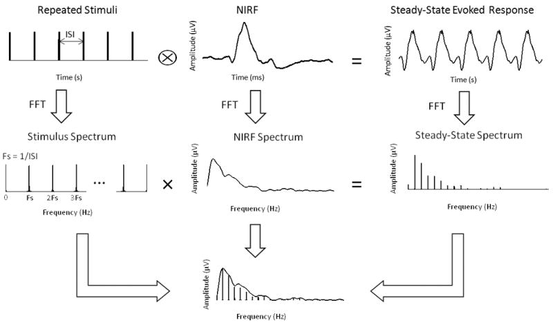
In the present study, the cascaded interactions between stimuli and neural and hemodynamic responses were modeled using linear systems. These models provided the theoretical hypotheses that were tested against the electroencephalography (EEG) and blood oxygen level dependent (BOLD) functional magnetic resonance imaging (fMRI) data recorded from human subjects during prolonged periods of repeated visual stimuli with a variable setting of the inter-stimulus interval (ISI) and visual contrast. Our results suggest that (1) neural response is nonlinear only when ISI<0.2 s, (2) BOLD response is nonlinear with an exclusively vascular origin when 0.25<ISI<4.2 s, (3) vascular response nonlinearity reflects a refractory effect, rather than a ceiling effect, and (4) there is a strong linear relationship between the BOLD effect size and the integrated power of event-related synaptic current activity, after modeling and taking into account the vascular refractory effect. These conclusions offer important insights into the origins of BOLD nonlinearity and the nature of neurovascular coupling, and suggest an effective means to quantitatively interpret the BOLD signal in terms of neural activity. The validated cross-modal relationship between fMRI and EEG may provide a theoretical basis for the integration of these two modalities.

Fig. 1

A) Diagram of the linear system models. Repeated stimuli are modeled as a train of delta functions, Σ_nδ(t-nΔ). Neural impulse response function represents the synaptic current activity, s(r,t), specific to a location r within the brain, induced by a single stimulus. s²(r,t) represents the power of the neural impulse response. If neural response is linear, the steady-state neural response evoked by the repeated stimuli, denoted as g(r,t), can be derived from the stimuli as g(r,t)=Σ_nδ(t- nΔ)*s(r,t). If neural and hemodynamic responses are coupled in a linear manner, the BOLD response can be represented by convolving the power (or magnitude) of the evoked neural response, g²(r,t), with the hemodynamic impulse response function, h(t), plus noise f_n(r,t). See Equations (1) through (5) in the text. These relationships rely on the assumptions of two linear time-invariant systems, which may be affected by the possible nonlinearities in both neural and vascular responses. B) Diagram of the system models after adding a nonlinear component, in terms of the ISI, to the linear system illustrated in A). This nonlinear component corrects the vascular refractory effect (see the Results section for more details).

Fig. 2

Neural response linearity/nonlinearity. a. Example of a 1-s period of the SSVEP signal measured from Oz is shown in blue. Corresponding linear prediction, derived by convolving the stimuli with the VEP signal at Oz, is shown in red. Vertical dashed lines represent the onsets of 4-Hz visual stimuli. b. Amplitude spectrum of the predicted SSVEP (red curve). c. Amplitude spectrum of the SSVEP measured from Oz (blue curve). Spatial distribution of the SSVEP amplitudes at the stimulus frequency (4 Hz) and its harmonic frequencies (8, 12, 16, 20, 24 Hz) are shown as 3-D scalp maps. d. Scatter-plot of the RCC values obtained from individual subjects at various ISIs (displayed as different symbols). An exponential function fitting the RCC-ISI values is illustrated by a curve in green. Vertical dashed line represents a neural refractory period of 200 ms. As such, neural response to repeated stimuli with ISI>200 ms is approximately linear (0.95<RCC≤1.01). When ISI<200 ms, the steady-state neural response is nonlinear (RCC<0.95). The shorter the ISI, the larger the degree of neural response nonlinearity.

Fig. 3

BOLD nonlinearity. a. ROI (surrounded by the green line) selected from the fMRI activation (red-to-yellow) within the upper calcarine sulcus, in response to stimuli presented in the lower-right quadrant of the visual field. b. Group-averaged (n=10) fMRI signals within the ROI shown in a, generated by a 30-s block of stimuli with ISIs from 0.25 to 6 s, are shown in blue. Corresponding regressors, derived by convolving the stimuli with the HRF, are shown in red. c. Steady-state heights of the measured fMRI signals (blue) and the corresponding regressors (red) are plotted as functions of the ISI, after normalizing (to 1) both the measured and modeled steady-state heights when ISI=6 s. d. Ratio between the measured fMRI signal and the regressor (i.e. the BOLD effect size) is plotted as a function of the ISI. Circles represent the group means. Error bars represent the standard errors of the mean (s.e.m) across subjects. The BOLD responses are approximately linear when ISI>4 s (marked by the vertical dashed line). When ISI<4 s, the BOLD responses are nonlinear. The shorter the ISI, the larger the degree of BOLD nonlinearity.

Fig. 4

Theoretical comparison between the BOLD-fMRI responses to a 30-s block of 100% (left) and 10% (right) stimuli with various contrasts and ISI, when assuming the BOLD response linearity. These plots are based on the results from computer simulations by assuming the single-stimulus evoked BOLD response amplitude (i.e. the HRF amplitude) for 10% contrast is half as large as that for 100% contrast (as shown in middle). The block BOLD responses (shown in bottom) derived by convolving the stimulus train with variable ISIs (as shown in top) with the respective HRF for both 100% and 10% contrast.

Fig. 5

Vascular ceiling vs. refractory effect. a. Group-averaged (n=10) BOLD effect sizes estimated from the measured fMRI signals within V1 in response to stimuli with various ISIs and a 100% (blue) or 10% (pink) visual contrast. b. Theoretical predictions of the BOLD effect sizes at various ISIs in response to 100% or 10% stimuli, by assuming a BOLD ceiling effect. c & d. Curves shown in c and d correspond to the curves shown in a and b, respectively, after normalizing (to 1) the corresponding means of the BOLD effect sizes when ISI≥4 s. e. Scatter-plot of the individual subjects' BOLD effect sizes, normalized in the way described as above, for both the 10% and 100% visual contrasts. A piece-wise linear function fitting all of the points is illustrated by two segments of green lines separated at ISI=4.2 s, which represents the vascular refractory period. Error bars in b and c represent the s.e.m. across subjects.

Fig. 6

fMRI-EEG coupling. a. BOLD-fMRI signals within V1, induced by a sustained period (30-s, marked by a light blue rectangle) of 2-Hz visual stimuli with seven different contrasts. b. VEP signals at Oz evoked by a single stimulus with variable contrasts. Vertical dashed line represents the stimulus onset. c. fMRI-seeded dipole model. Locations of five dipoles (left) were initiated to the centers of the corresponding ROIs selected from the fMRI activation map (right, p<0.01 corrected). Red-circled dipole represents the dipole in V1. d. Estimated V1 dipole source activity for different contrasts. e & f. Scatter-plot of the BOLD effect sizes within V1 and the integrated power (e) or magnitude (f) of the V1 dipole source, for different visual contrasts. Red lines illustrate linear functions that fit the corresponding scatter points. Data shown in this figure are the average across subjects (n=10). g. Correlations between the BOLD effect size and the integrated source power or magnitude within various post-stimulus periods (0∼150 ms to 0∼500 ms). In a, b and d, visual contrasts are color-coded in a way specified in a.

Fig. 7

Illustration of the SSVEP spectral analysis. When the steady-state evoked response can be expressed as the result of convolving the stimuli with an equivalent neural impulse response function, the frequency spectrum of the steady-state evoked response equals the spectrum of the stimuli multiplied by the spectrum of the impulse response. By dividing the spectrum of the steady-state evoked response by the stimulus spectrum at the multiples of the stimulus frequency, discrete samples of the impulse response function represented in the frequency domain were obtained. The summation of these discrete samples represents the discrete integral of this spectral profile.

References

-
- Allen PJ, Josephs O, Turner R. A method for removing imaging artifact from continuous EEG recorded during functional MRI. Neuroimage. 2000;12:230–239. - PubMed
- Allen PJ, Polizzi G, Krakow K, Fish DR, Lemieux L. Identification of EEG events in the MR scanner: The problem of pulse artifact and a method for its subtraction. Neuroimage. 1998;8:229–239. - PubMed
- Arthurs OJ, Williams EJ, Carpenter TA, Pickard JD, Boniface SJ. Linear coupling between functional magnetic resonance imaging and evoked potential amplitude in human somatosensory cortex. Neuroscience. 2000;101:803–806. - PubMed
- Attwell D, Iadecola C. The neural basis of functional brain imaging signals. Trends Neurosci. 2002;25:621–625. - PubMed
- Bandettini PA, Wong EC, Hinks RS, Tikofsky RS, Hyde JS. Time course EPI of human brain function during task activation. Magn Reson Med. 1992;25:390–397. - PubMed
Publication types
MeSH terms
Substances
Grants and funding
LinkOut - more resources
Full Text Sources