A neurophysiologically plausible population code model for feature integration explains visual crowding

Abstract

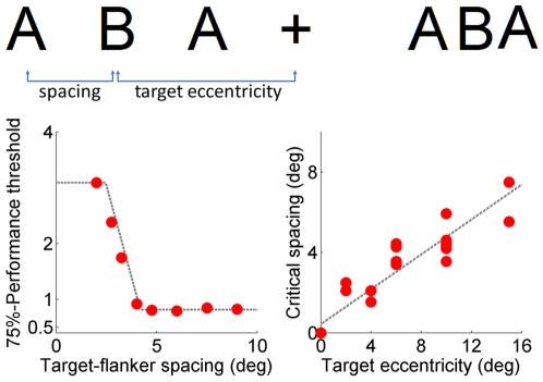
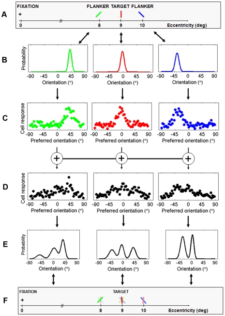
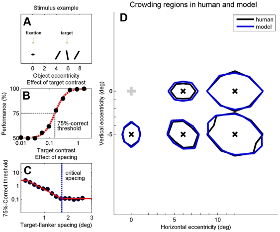
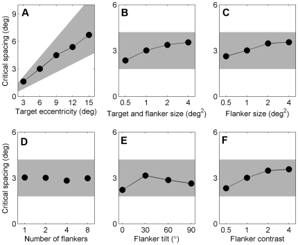
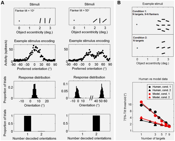
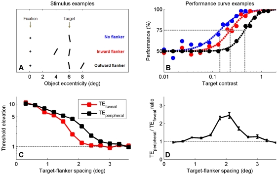
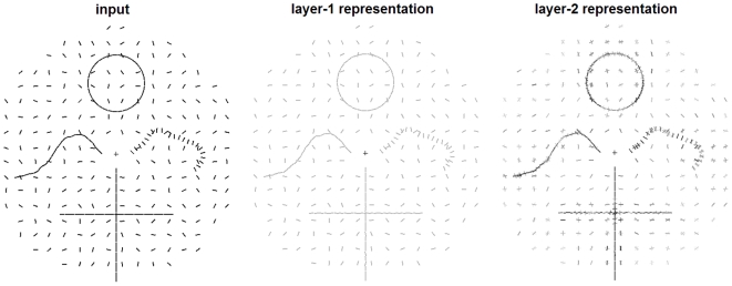
An object in the peripheral visual field is more difficult to recognize when surrounded by other objects. This phenomenon is called "crowding". Crowding places a fundamental constraint on human vision that limits performance on numerous tasks. It has been suggested that crowding results from spatial feature integration necessary for object recognition. However, in the absence of convincing models, this theory has remained controversial. Here, we present a quantitative and physiologically plausible model for spatial integration of orientation signals, based on the principles of population coding. Using simulations, we demonstrate that this model coherently accounts for fundamental properties of crowding, including critical spacing, "compulsory averaging", and a foveal-peripheral anisotropy. Moreover, we show that the model predicts increased responses to correlated visual stimuli. Altogether, these results suggest that crowding has little immediate bearing on object recognition but is a by-product of a general, elementary integration mechanism in early vision aimed at improving signal quality.

Figure 1. An example demonstrating the crowding phenomenon.

Top: The two B's are at equal distance from the fixation cross. On the left, where the center-to-center spacing between the letters is approximately one half of the eccentricity of the central letter, the “B” can easily be recognized when fixating the cross. Letter spacing on the right is much smaller, and the “B” appears to be jumbled with its neighbors. Bottom, left: Human data from a typical crowding experiment. Crowding diminishes as target-flanker spacing is increased, up to a certain critical spacing after which flankers have no effect. Bottom, right: Findings from psychophysical studies show that critical spacing is a linear function of target eccentricity. Data from .

Figure 2. A graphical illustration of our model.

A. In this example, the input consists of three oriented bars (the colors are only for visualization purposes and not part of the input to the model); B. Probability distributions are defined for the input stimuli; these distributions capture the stimulus uncertainty caused by neural noise in processing stages prior to the first layer of the model; C. In the first layer, a neural representation is computed for each of these distributions; D. In the second layer, the stimulus representation at each location is integrated with the representations of stimuli at neighboring locations. Integration is implemented as a weighted summation, such that nearby stimuli receive higher weights than stimuli that are far away; E. The resulting population codes are decoded to a mixture of normal distributions, with each component representing a perceived orientation at the respective location; F. Due to integration, the resulting percept of closely spaced stimuli will be crowded.

Figure 3. Comparison of crowding regions reported for humans with crowding regions estimated by our model.

A. The input stimulus on each trial consisted of a ±10° tilted target stimulus and two 30° tilted flankers placed on opposite sides of the target. If the sign of the post-integration stimulus representation associated with the target position was the same as the sign of the input target, then performance on that trial was considered correct; B. Performance was estimated for a range of target contrasts, yielding a curve that is very similar to psychometric curves typically found with human experiments (compare, for example, with data shown in Figure 1). Based on these curves, contrast thresholds were estimated that produce 75% correct performance; C. Contrast thresholds decrease as target-flanker spacing is increased. The smallest spacing at which the flankers do not have an effect is defined as the critical spacing; D. Critical spacings were estimated in several directions around the target, at five different target positions. These simulation data accurately reproduce the critical regions measured psychophysically in humans. Human data from .

Figure 4. Simulation results showing the effect of several stimulus manipulations on estimated critical spacing.

The shaded areas represent the range of critical spacings that are typically reported in the literature (0.3–0.6 times target eccentricity). Standard errors are smaller than the marker size. A. Critical spacing scales linearly with target eccentricity; B–F. Critical spacing is only weakly affected by various stimulus manipulations. The eccentricity of the target was 6 degrees in these experiments.

Figure 5. Compulsory averaging of crowded orientation signals explained as the result of ‘merging’ population codes.

A. Simulation results illustrating how the ‘compulsory averaging’ effect arises in our model. Top row: example input stimuli, consisting of a vertical target flanked by two equally tilted flankers. Second row: single trial examples of population codes representing the post-integration stimulus at the target position. Third row: distributions of the orientations encoded at the target locations after integration (1000 trials). Bottom row: corresponding distributions of the number of perceived stimuli at the target position. When target and flanker tilt are nearly identical, their population code representations merge into a single hill of activity when integrated. The resulting code is decoded to a single orientation, with a value intermediate between the values of the input stimuli. This effect diminishes when the difference between target and flanker tilt is increased; B. Model fit to human psychophysical data. Top: Example stimuli of the experiment described in . The task was to report the tilt direction of a variable number of equally tilted targets positioned within a set of horizontal flankers. Bottom: Identification thresholds predicted by our model are very close to those found for human subjects. Human data from , subject LP.

Figure 6. Simulation results illustrating the anisotropic effects of foveal vs peripheral flankers on target identification.

A. Stimuli consisting of a ±10° tilted target, flanked by either no flanker, a foveal flanker, or a peripheral flanker. B. Both flankers elevate target tilt identification thresholds, but this effect is largest for peripheral flankers. We define threshold elevations TE_foveal and TE_peripheral as the 75%-correct target contrast found for the condition with a foveal and peripheral flanker, respectively, divided by the 75%-correct target contrast found for the condition without a flanker. C. Predicted threshold elevations plotted as a function of target-flanker spacing. When target-flanker spacing is small or when it approaches the critical spacing, the effects of foveal and peripheral flankers are comparably strong. However, in the intermediate range, a peripheral flanker produces larger threshold elevations (i.e., stronger crowding) than a foveal flanker. D. The same data as in C, but now shown as a ratio (i.e., the values at black data points from panel C divided by those at the red data points).

Figure 7. Simulation results showing how our model responds to visual contours.

Left image: input stimulus, consisting of a set of oriented line segments comprising several contours within a noisy background. The ‘+’ symbol indicates the center of the visual field and was not part of the stimulus. Central image: a visualization of the stimulus representation in the first layer of our model, which is a noisy version of the input. The contrast of the bars is set to the median of the contrasts in the right image. Right image: a visualization of the decoded stimulus representations after integration. At every original input location, the post-integration population code was decoded to a mixture of normal distributions. The contrast of each bar is proportional to the associated mixing proportion. Note the highlighting of the contours and the crowding effects in the periphery, which agrees well with the subjective experience when viewing the input stimulus.

References

1. Korte W. Über die Gestaltauffassung im indirekten Sehen. Zeitschrift für Psychologie. 1923;93:17–82.
1. Stuart JA, Burian HM. A study of separation difficulty. Its relationship to visual acuity in normal and amblyopic eyes. Am J Ophthalmol. 1962;53:471–477. - PubMed
1. Pelli DG, Tillman KA. The uncrowded window of object recognition. Nat Neurosci. 2008;11:1129–1135. - PMC - PubMed
1. Levi DM. Crowding–an essential bottleneck for object recognition: a mini-review. Vision Res. 2008;48:635–654. - PMC - PubMed
1. Bouma H. Interaction effects in parafoveal letter recognition. Nature. 1970;226:177–178. - PubMed
Publication types