IVGTT glucose minimal model covariate selection by nonlinear mixed-effects approach

Abstract

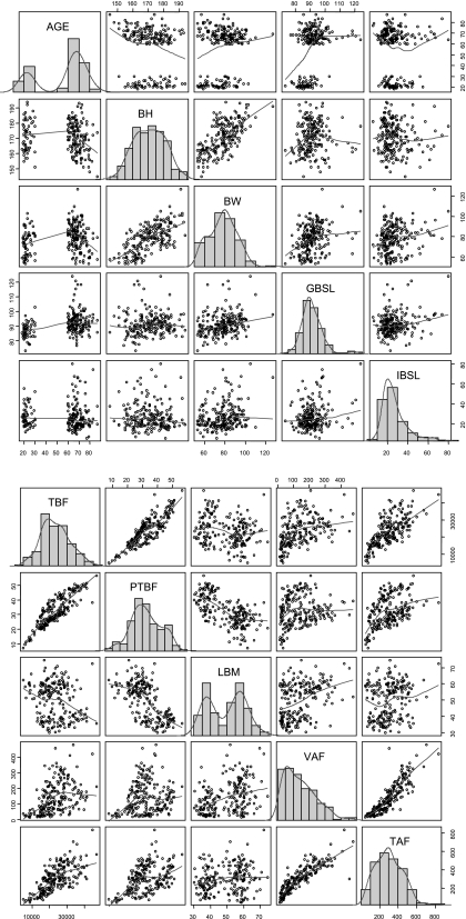
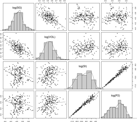
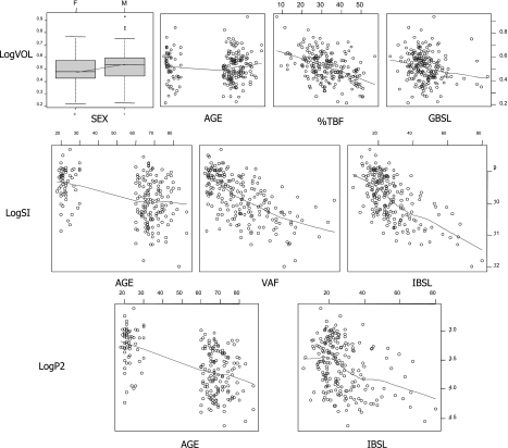
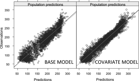
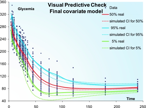
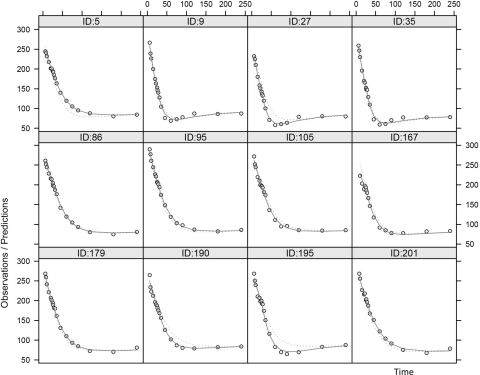
Population approaches, traditionally employed in pharmacokinetic-pharmacodynamic studies, have shown value also in the context of glucose-insulin metabolism models by providing more accurate individual parameters estimates and a compelling statistical framework for the analysis of between-subject variability (BSV). In this work, the advantages of population techniques are further explored by proposing integration of covariates in the intravenous glucose tolerance test (IVGTT) glucose minimal model analysis. A previously published dataset of 204 healthy subjects, who underwent insulin-modified IVGTTs, was analyzed in NONMEM, and relevant demographic information about each subject was employed to explain part of the BSV observed in parameter values. Demographic data included height, weight, sex, and age, but also basal glycemia and insulinemia, and information about amount and distribution of body fat. On the basis of nonlinear mixed-effects modeling, age, visceral abdominal fat, and basal insulinemia were significant predictors for SI (insulin sensitivity), whereas only age and basal insulinemia were significant for P2 (insulin action). The volume of distribution correlated with sex, age, percentage of total body fat, and basal glycemia, whereas no significant covariate was detected to explain variability in SG (glucose effectiveness). The introduction of covariates resulted in a significant shrinking of the unexplained BSV, especially for SI and P2 and considerably improved the model fit. These results offer a starting point for speculation about the physiological meaning of the relationships detected and pave the way for the design of less invasive and less expensive protocols for epidemiological studies of glucose-insulin metabolism.

Fig. 1.

Overview of covariate values. Histogram plots and smoothed densities for the covariate set (see also Table 1). Regressions between the most correlated covariates are also shown, and a smoothed tendency line is superimposed to depict the trend of the relation. A: AGE, age; BH, body height; BW, body weight; GBSL, basal glucose level; IBSL basal insulin level. B: TBF, total body fat; PTBF, %TBF; LBM, lean body mass; VAF, visceral abdominal fat; TAF, total abdominal fat.

Fig. 2.

Overview of individual parameter values from base model. Scatterplots and histograms of the logarithm of the individual parameter values, as obtained with the base model. SG, glucose effectiveness; VOL, apparent volume of glucose distribution per unit of body mass; SI, insulin sensitivity; P2, insulin action. The correlation is apparent between log(SI) and log(P2) and between log(SG) and log(VOL), as accounted for by the relative terms in the covariance matrix Ω.

Fig. 3.

Individual parameters vs. significant covariates. Scatterplots with the logarithm of the parameter values obtained with the base model regressed vs. the respective covariates included in the final model.

Fig. 4.

Observations vs. population predictions. Scatterplot of the observations (DV) vs. population predictions (PRED) for the base model (left) and the final covariate model (right).

Fig. 5.

Visual predictive check. Visual predictive check (3,000 simulations) obtained with the final covariate model. The confidence interval (CI) for the 5, 50, and 95% percentiles for simulated (dashed lines) and real data (solid lines) are displayed.

Fig. 6.

Individual profiles. Individual predictions vs. time for some randomly selected subjects. ID, subject ID number. Dots represent observed concentrations; dashed line is the population prediction; solid line is the individual prediction.

References

-
- Agbaje OF, Luzio SD, Albarrak AI, Lunn DJ, Owens DR, Hovorka R. Bayesian hierarchical approach to estimate insulin sensitivity by minimal model. Clin Sci (London) 105: 551–560, 2003. - PubMed
- Basu R, Breda E, Oberg AL, Powell CC, Dalla Man C, Basu A, Vittone JL, Klee GG, Arora P, Jensen MD, Toffolo G, Cobelli C, Rizza RA. Mechanisms of the age-associated deterioration in glucose tolerance: contribution of alterations in insulin secretion, action, and clearance. Diabetes 52: 1738–48, 2003 - PubMed
- Basu R, Dalla Man C, Campioni M, Basu A, Klee G, Toffolo G, Cobelli C, Rizza RA. Effects of age and sex on postprandial glucose metabolism: differences in glucose turnover, insulin secretion, insulin action, and hepatic insulin extraction. Diabetes 55: 2001–2014, 2006 - PubMed
- Beal S, Sheiner L, Boeckmann A. NONMEM Users Guides (1989–2006). Ellicott City, MD: ICON Development Solutions
- Beal SL, Sheiner LB. Estimating population kinetics. Crit Rev Biomed Eng 8: 195–222, 1982 - PubMed
Publication types
MeSH terms
Substances
LinkOut - more resources
Full Text Sources