Dichotomy of functional organization in the mouse auditory cortex

Abstract

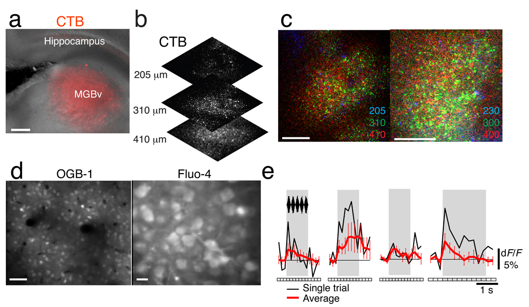
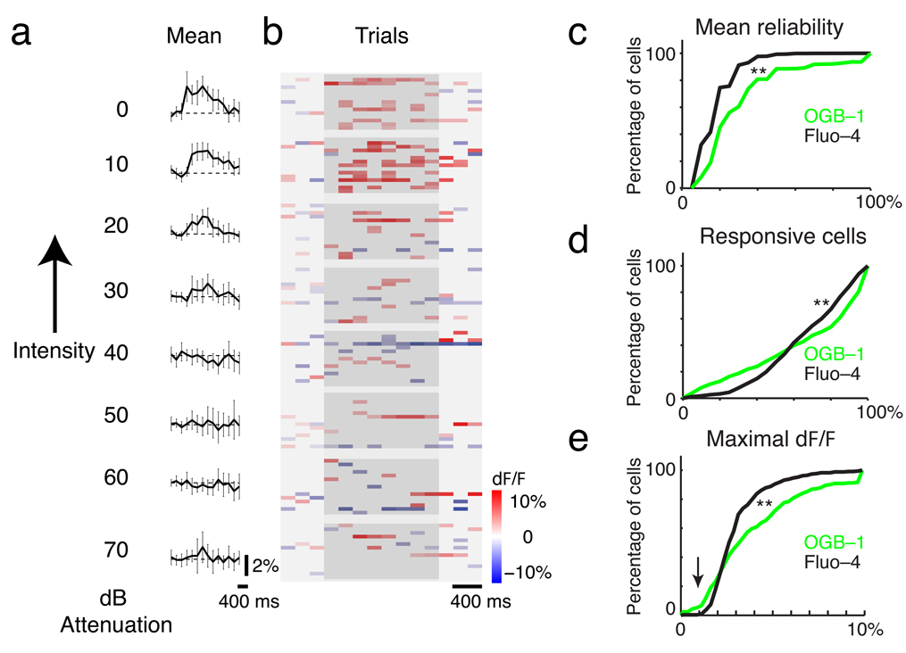
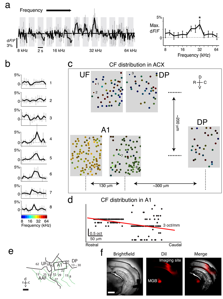
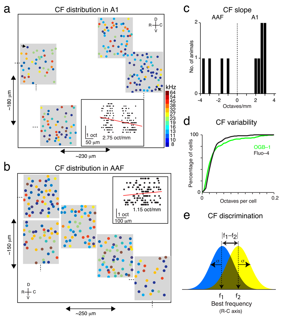
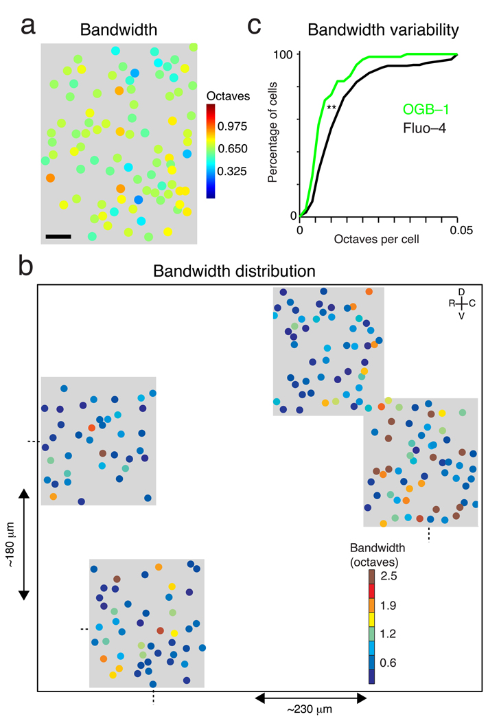
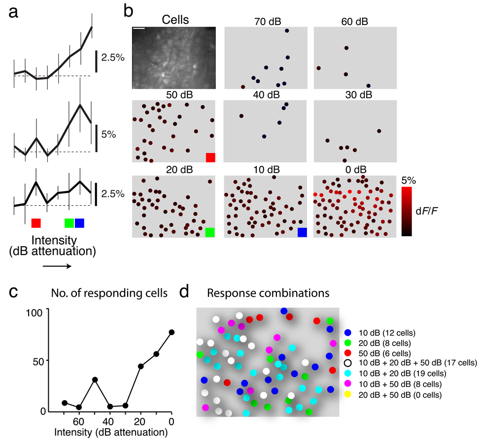
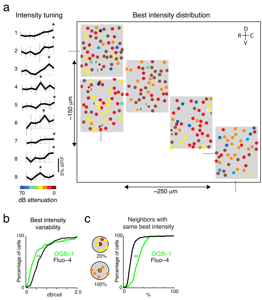
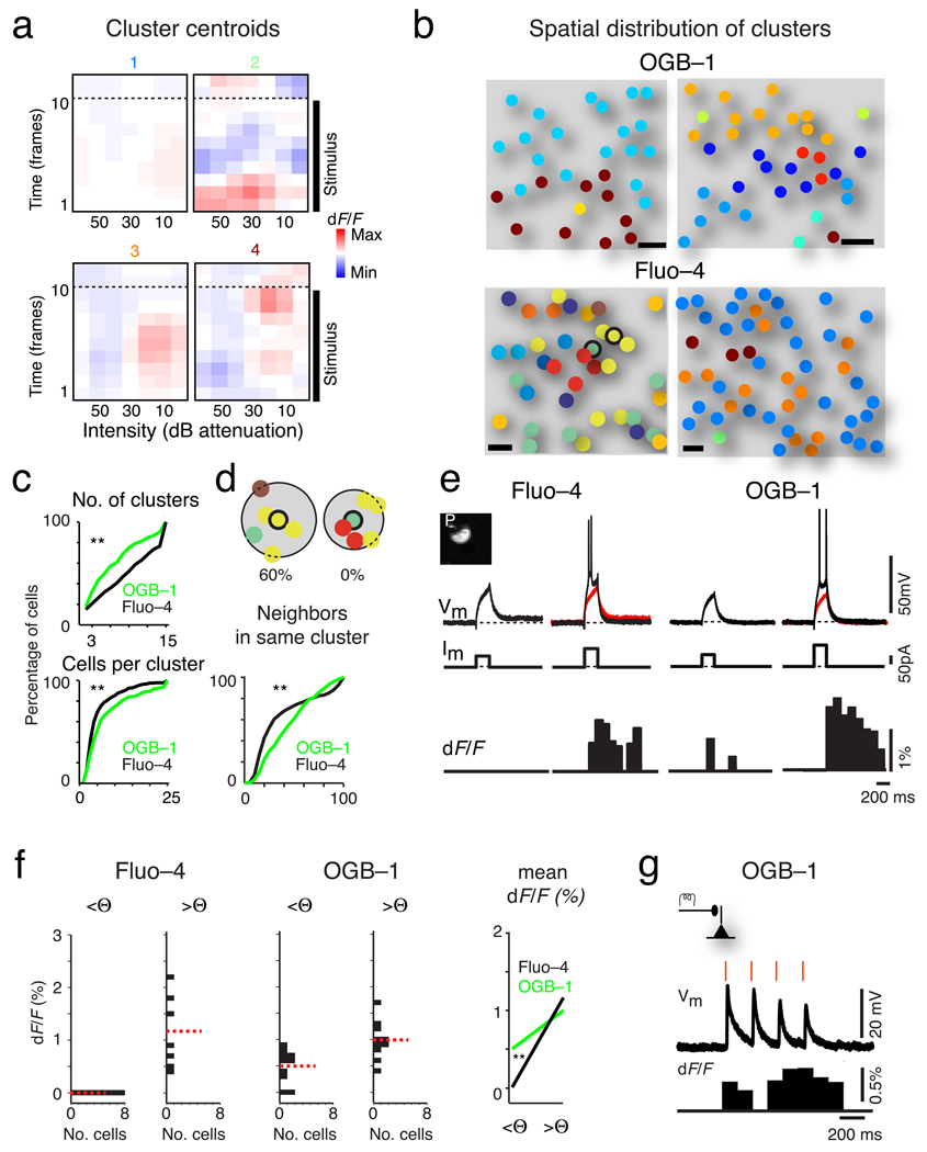
The sensory areas of the cerebral cortex possess multiple topographic representations of sensory dimensions. The gradient of frequency selectivity (tonotopy) is the dominant organizational feature in the primary auditory cortex, whereas other feature-based organizations are less well established. We probed the topographic organization of the mouse auditory cortex at the single-cell level using in vivo two-photon Ca(2+) imaging. Tonotopy was present on a large scale but was fractured on a fine scale. Intensity tuning, which is important in level-invariant representation, was observed in individual cells, but was not topographically organized. The presence or near absence of putative subthreshold responses revealed a dichotomy in topographic organization. Inclusion of subthreshold responses revealed a topographic clustering of neurons with similar response properties, whereas such clustering was absent in supra-threshold responses. This dichotomy indicates that groups of nearby neurons with locally shared inputs can perform independent parallel computations in the auditory cortex.

Figure 1. Functional 2-photon Ca²⁺ imaging in mouse ACX

a–c: Confirmation of craniotomy and imaging site in ACX by anterograde labeling. Choleratoxin-B was injected into the MGB stereotactically (a). A craniotomy was performed at our imaging locations. Fluorescently labeled terminals were imaged at 3 depths of 205, 310 and 410 µm from the cortical surface (b). Following imaging of terminals in vivo slices were cut to confirm tracer injection in the MGB (a). c: Superposition of images taken at different depths in 2 animals are shown. Note that most signals originated at 300–400 µm depth indicating the thalamo-recipient layer. Thus our imaging location is in A1. Scale bars in a and c: 100 µm. d: Shown are images of bulk loading ACX with OGB–1 (left) and Fluo–4 (right). The area over which cells were loaded varied in experiments from 200 µm to 1 mm diameter regions. Scale bars are 50 µm (left) and 10 µm (right) e: Shown are single trial (black) and mean (red) fluorescence changes (dF/F) with SAM broadband noise from 4 different cells. Errorbars show 95% confidence intervals indicating a significant fluorescence change. Frame timing is shown below fluorescence trace.

Figure 2. ACX Ca²⁺ responses are unreliable

a: Traces show mean fluorescence changes (dF/F) in one cell for SAM noise of varying intensity. Significant responses at 0–30 dB attenuations were seen in this case. Errorbars show 95% confidence intervals. b: Thresholded fluorescence changes (dF/F) (colorbar to right) in all individual trials for the same cell. Gray backgrounds depict stimulation period. Note the unreliability but larger dF/F of single trials. c: Cumulative distribution of mean reliability in all imaged cells with Fluo–4 (black) and OGB–1 (green). Mean reliability was defined as the fraction of trials with significant responses (methods) in each cell for a set of stimuli (either different intensities of SAM noise or different frequencies of SAM tone or noise or tone pips). d: Cumulative distribution of the fraction of responsive cells in each imaged field (same animals as in c). A responsive cell was defined as a cell that responded at least to one of the presented stimuli significantly (95% confidence interval). e: Cumulative distribution of maximum response in each field. Mean maximum response is higher with OGB–1 (4.8%) than Fluo–4 (3.3%, p<0.05, t-test, same animals as in c and d).

Figure 3. Large scale organization of ACX probed with single cell resolution

a: Traces show responses (dF/F) of single neurons in A1 to SAM tones of various stimulus frequencies (duration indicated by gray area). Plotted is the mean response with 95% confidence intervals. Right: Plotting peak dF/F versus stimulation frequency (tuning curve) shows unimodal tuning (CF = 32 kHz, ‘*’). b: Tuning curves from 8 cells imaged in one animal (locations indicated in c). CF progresses from cell 4 to 8. c: Reconstructions of the large-scale organization of ACX in one animal by imaging multiple sites. The relative distances (approximate) between centers of imaged sites (gray boxes) are indicated. Relative positions not to scale. Color denotes CF (colorbar in b) based on peak dF/F and luminance response strength. E.g. cells tuned to 38 kHz are orange. Strongly responding cells are bright orange, while weakly responding cells are dark orange. Different regions of ACX are identified based on CF and tuning curve shape (b): A1, DP and UF. d: Progression of cell CF as a function of rostro-caudal position. Red line indicates best fit. e: Large-scale organization of mouse ACX redrawn from . Box indicates putative location of imaging site in A1 (c). Because of inter-animal variation exact positions of UF and DP relative to A1 in c are slightly different. This is a rough depiction as clear demarcations of the different regions are lacking. Scale bar = 250 µm. f: Post-hoc verification of A1 imaging site (c) by DiI injection. MGB is retrogradely labeled. Damage on imaging site is from DiI crystal insertion after imaging. Scale bar = 1 mm.

Figure 4. Tonotopy exists in A1 and AAF on large but not on small spatial scales

a: Reconstruction of 4 imaging sites (relative positions are approximate) in A1 in one animal. Cell CF is indicated by color and increases from caudal (~ 10 kHz) to rostral (~ 23 kHz). Cells at opposite A1 ends can show similar CF’s (arrows). Positive CF gradient (inset) indicates that imaging site was in A1. b: Reconstruction of 5 imaging sites (relative positions are approximate) in ACX in one animal (different from a). Negative CF gradient (maximum slope after rotation and exclusion of neurons that were in secondary region, inset) indicates that imaging site was in AAF. c: Slope of CF gradient in rostro-caudal direction from fits to CFs and their respective cells’ location (see a, b, and Fig. 3d). Due to inter animal variability and slight differences in animal position, the CF gradient that was fit could occur at an angle from the rostro-caudal axis. Positive or negative CF slopes characterize A1 or AAF respectively. Since not the entire extent of ACX was covered in each animal CF slopes are an estimate of the large-scale CF progression. d: Cumulative distribution of CF variability (standard deviation of CF normalized by number of cells in imaged field) within ACX. Variability (median 0.025 octaves/cell, 34 cells per site, average 0.85 octaves per ~ 100µm²) was similar for OGB–1 and Fluo–4 (P > 0.1; OGB–1 n = 15; Fluo–4 n = 24 animals). e: d' analysis of sharpness of tonotopy. d' is the mean CF difference at different A1 locations normalized by the standard deviation. d' = 1 indicates that mean CFs can be discriminated.

Figure 5. High local variability in bandwidth

a: Color-coded plot of bandwidth variation in A1 for the leftmost field in Fig. 3c shows varied bandwidth in nearby cells. Scale bar = 20 µm. b: Large-scale reconstruction of bandwidths is shown for the area imaged for the example in Fig. 4a; this case shows similar heterogeneity of bandwidths as in Fig. 5a. c: Cumulative distribution of variability of bandwidth within imaging sites shows that variability was lower for cells imaged with OGB–1 than with Fluo–4 (0.007 and 0.01, P < 10⁻⁴, ‘**’, n = 15 animals with OGB–1 and 24 animals with Fluo–4). Variability was measured as the standard deviation of bandwidths normalized by the number of cells in the field of view.

Figure 6. Intensity tuning and local heterogeneity in noise responses

a: Traces show maximum mean fluorescence changes to SAM noise stimuli with increasing intensity (decreasing attenuation) in 3 cells. Cells can show monotonic (top) and nonmonotonic (middle and bottom) intensity tuning curves. Nonmonotonic tuning curves were identified by a significant decrease in dF/F at higher intensities. Errorbars show 95% confidence intervals. b: Plotted are cells in one imaging site (top left) that responded to noise at a particular intensity (‘activation plot’). Intensity levels are given as dB attenuation. Brightness of circles indicates response strength (maximum mean dF/F) (colorbar, right). Note that different populations of cells responded at each intensity. cale bar shows 20 µm c: Shown is the number of cells activated at various intensities indicating a nonmonotonic population representation of sound intensity. d: Shown is the superposition of 3 of the activation plots in b identified by colored squares. Colors of cells depict which combination of the 3 (red, green and blue squares) intensities a cell responded (example white – all 3 intensities, cyan – green and blue intensities). Note that the response properties of nearby cells are heterogeneous.

Figure 7. Figure 7. Lack of organized intensity maps

a: Reconstruction of 5 imaging sites in ACX (boxes) of one animal depicting the best intensities of cells in response to SAM broadband noise. The colors of the circles indicate the preferred intensity (colorbar). There is no clear pattern of organization of best intensities. Traces on left show intensity functions of 9 cells indicated in the reconstruction. '*' denotes the best intensity. Note that some cells showed monotonic while others showed nonmonotonic intensity functions. b: Cumulative distribution of best intensity variability within an imaging site. Variability was lower for cells imaged with OGB–1 than those imaged with Fluo–4 (P < 10⁻⁵, ranksum, ‘**’, n = 15 animals with OGB–1 and 24 animals with Fluo–4). Values were normalized by the number of cells in the field of view. c: Cumulative population distribution of average percentage of cells in 5 neighboring cells in a field of view that had the same preferred intensity as the central cell. OGB–1 showed more (P < 10⁻¹⁰) percentage of cells on average (30%) had same preferred intensity as the central cell than with Fluo–4 (15%). Cartoon on the left shows how the local percentages were computed (same population as in b).

Figure 8. ACX cells receive shared inputs but respond differentially

a: Mean response characteristics (centroids) of 4 clusters formed in b (lower right image, label color indicates cluster). b: Examples of cluster formation to SAM tone or noise sets with OGB–1 (upper) and Fluo–4 (lower). Cells in each cluster have same color. The within to inter cluster distance ratios indicating degree of cluster separation are 0.358, 0.988 for OGB–1 and 0.871, 0.590 for Fluo–4. c: Cumulative distributions of cluster number and size (P < 0.05 ‘**’, n = 15 animals with OGB–1, n = 24 with Fluo–4). d: Fraction of neighbors in same cluster (numbers of cells within the same cluster from the 5 nearest neighbors). Analysis illustrated (top) for 2 cells in b (bottom left, black circles). Cumulative distributions (bottom) are different (KS-test, P < 10⁻⁸, same animals as c). e: In vitro current-clamp recordings and 2-photon imaging of 2 cells filled with Fluo–4 and OGB–1 respectively. Inset shows image of one recorded cell ('P': patch pipette). Traces show membrane voltage (V_m, upper), current (I_m, middle), and significant (outside 95% confidence interval) mean dF/F (10 repeats, lower). Red traces show the respective subthreshold depolarization (left) in suprathreshold traces. f: Distributions of in vitro dF/F for the 2 categories for each cell (OGB–1 n = 10, Fluo–4 n = 7 cells): highest subthreshold depolarization tested and spiking. Means indicated by red lines. Peak depolarization (22 ± 5 mV and 23 ± 7 mV respectively, P = 0.65) and membrane charging times for OGB–1 and Fluo–4 were similar (P > 0.5). g: Traces show V_m (top) and mean dF/F (bottom, 20 repeats) during electrical stimulation (4 pulses, red lines) of horizontal inputs (cartoon).

References

1. Mountcastle VB. The columnar organization of the neocortex. Brain. 1997;120(Pt 4):701–722. - PubMed
1. Hubel DH, Wiesel TN. Ferrier lecture. Functional architecture of macaque monkey visual cortex. Proc R Soc Lond B Biol Sci. 1977;198:1–59. - PubMed
1. Schreiner CE, Winer JA. Auditory cortex mapmaking: principles, projections, and plasticity. Neuron. 2007;56:356–365. - PMC - PubMed
1. Koulakov AA, Hromadka T, Zador AM. Correlated connectivity and the distribution of firing rates in the neocortex. J Neurosci. 2009;29:3685–3694. - PMC - PubMed
1. Hromadka T, Deweese MR, Zador AM. Sparse representation of sounds in the unanesthetized auditory cortex. PLoS Biol. 2008;6:e16. - PMC - PubMed
Publication types