

doi: 10.1016/j.pnmrs.2008.04.001.
Optimization of static magnetic field homogeneity in the human and animal brain in vivo
Affiliations
- PMID: 20126515
- PMCID: PMC2802018
- DOI: 10.1016/j.pnmrs.2008.04.001
Item in Clipboard
Optimization of static magnetic field homogeneity in the human and animal brain in vivo
Prog Nucl Magn Reson Spectrosc.
.
No abstract available
Figures
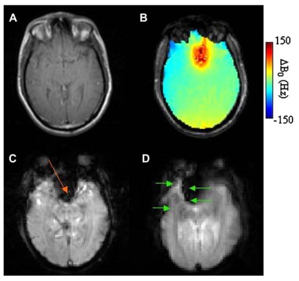
(A) Fast-spin-echo (FSE) anatomic image of an axial slice (6 mm thick) through the frontal cortex of the human brain at B0 = 3T. (B) ΔB0 field map over the same slice, (C) signal loss in weighted (TE = 35 ms) gradient-echo images (most prominent loss indicated with orange arrow), and (D) distortion in EPI images (indicated with green arrows), collected with TE = 25 ms, 64 × 64 in plane pixels over a 20 cm ×20 cm FOV, a readout bandwidth of 250 kHz. Arrows indicate directions of distortion in the phase-encoded dimension.

Water-suppressed proton spectra of two voxels, indicated in an axial MRI (B), where local field inhomogeneity (B0 =4T) is dramatically greater in one (anterior) of the voxels. Compared to the spectrum in the posterior voxel (C), spectral linewidths and water suppression are clearly degraded in the anterior voxel (D) due to the degraded field homogeneity in its locality. The presented field map (A) displays the field inhomogeneity causing increased linewidths and reduced water suppression in the anterior voxel.
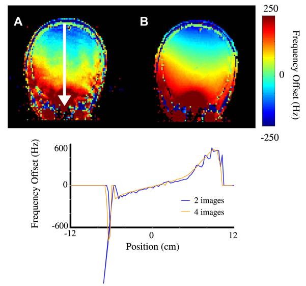
Axial field maps using (A) 1 delay whereby two images of τj = 0 and 0.33 ms are collected, and (B) using temporal unwrapping of 3 delays (4 images) with τi = 0, 0.33, 1.0 and 3.0 ms, and field traces as indicated by white arrows.

(A) Spin echo MRI at B0 = 4T used for susceptibility model construction, (B) susceptibility model showing air (white) and water (black) used for computational estimation of inhomogeneity, (C) experimental spin-echo field map of phantom, (D) computed field map, (E) difference map between measured and computed fields, (F) horizontal (x) traces as indicated through the phantom, and (G) vertical (z) traces as indicated through the phantom. Reproduced with permission from [6].

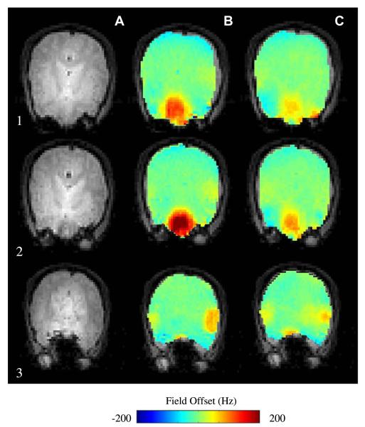
Two axial slices (1–2) and a central sagittal (3) slice showing (A) MRI, (B) experimental field maps, (C) computed field maps. Adapted with permission from [6].
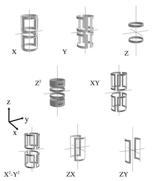
Shim coil designs for all first and second order shim coils. Notice that the tesseral shim terms are grouped in pairs rotated by 90° in the xy plane (i.e. ZY is a rotated ZX configuration). Illustrations courtesy of Dr. Dan Green, Magnex Scientific.
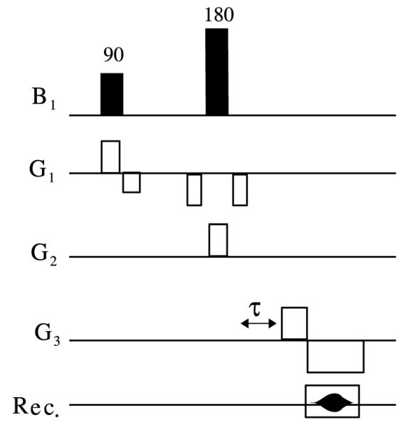
Pulse sequence for acquisition of FASTMAP linear projection field map. G1, G2 and G3 represent orthogonal oblique gradient vectors defining a given projection. As was described in Section 3.1, acquisitions must be made with two different timing parameters τ (typically τ = 0 and τ > 0). A slice selective 90° pulse brings magnetization in a given oblique slice down to the transverse plane and a 180° pulse then operates on a second slice intersecting the first slice. Readout occurs then in a direction perpendicular to both slice selection gradients.

(A) Axial MRI at B0 = 3T of two axial slices encompassing the sinus cavity region, residual inhomogeneity after (B) first order shimming, (C) with the inclusion of second-order shims, (D) with the inclusion of third-order shims.
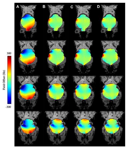
Coronal field inhomogeneity maps of the mouse brain at 9.4T with (A) no shimming, (B) first-order shimming, (C) first and second-order shimming, and (D) first through third-order shimming.
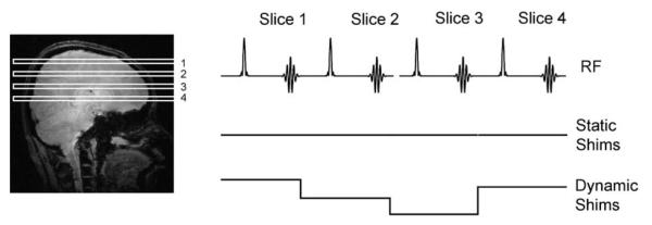
The principle of DSU in multi-volume acquisitions. As spins within individual slices are excited and sampled (top row), a static shim setting (middle row) would remain constant, while a dynamic shim setting (lower row) updates the currents in the shim amplifiers during each slice excitation and sampling.

Water spectra collected after 25% Z2 shim changes (A) without and (B) with shim-change pre-emphasis. Reproduced from [60] with permission of Wiley-Liss, Inc., a subsidiary of John Wiley and Sons, Inc.

Sagittal anatomic MRI provides voxel positioning in the interleaved multi-voxel MRS acquisition. (A) Water spectra (B0 = 4T, TE = 80 ms, TR = 2.5 s, 256 averages), acquired from the four voxels using a static global shim. (B) Water spectra acquired using DSU. Linewidths of the water spectra are as indicated. (C) 1H metabolite spectra collected using DSU. Reproduced from [62] with permission of Wiley-Liss, Inc., a subsidiary of John Wiley and Sons, Inc.

Homogeneity improvement with whole-slice optimized DSU. Field maps with (DSU) and without (global) dynamic shim changes along with slice-specific histograms for both shim settings. B0 = 4T.
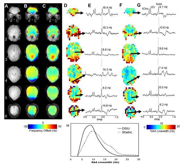
(A) Anatomic images of MRSI slices, (B) B0 maps without DSU, (C) with DSU, (D) NAA linewidths across viable MRSI voxels with DSU, (F) without DSU, (E) spectra from indicated voxels without DSU, and (G) with DSU. (H) Provides a histogram of viable NAA linewidths across all slices with and without DSU. Images obtained at B0 = 4T. Reproduced from [62] with permission of Wiley-Liss, Inc., a subsidiary of John Wiley and Sons, Inc.
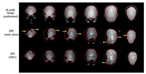
EPI images (64 × 64 in-plane pixels over 25.6 cm × 25.6 cm, 4 mm slices, B0 = 4T, TR = 2500 ms, TE = 25 ms, and readout bandwidth of 100 kHz) under static and dynamic second-order shim settings for axial slices (from left to right). Dotted lines indicate the brain contours as extracted from an undistorted FLASH acquisition (top row). Arrows designate areas of significant image quality improvement.
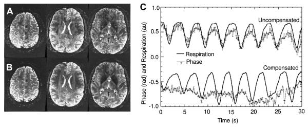
Axial sliced gradient echo images (B0 = 7T, TE 40 ms, TR = 500 ms) without (A) and with (B) respiration-compensated dynamic shimming. (C) Temporal plots of phase measured in a single imaging voxel and respiration. Without temporal DSU, there is a clear tracking of phase with the respiratory cycle. When temporal DSU is applied, the compensated phase has a much smaller dependence on the respiratory cycle. Results courtesy of Dr. Peter van Gelderen.
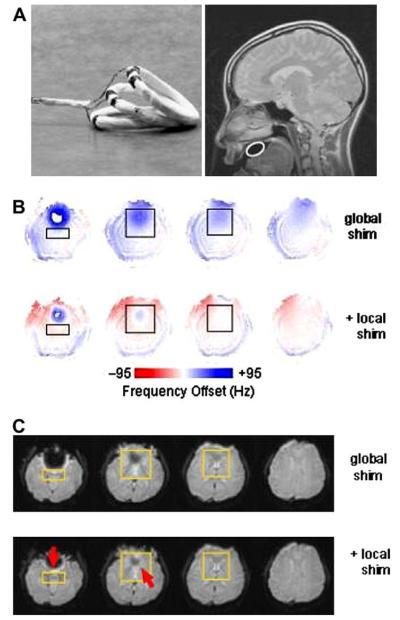
(A) Image and anatomic location of intra-oral local active shims. (B) Field-map results of optimized local active shim use. (C) Signal-recovery in gradient-echo imaging (TE = 40 ms, 5 mm slices) with the local shim assembly. B0 = 1.5T Reproduced from [75] with permission of Wiley-Liss, Inc., a subsidiary of John Wiley and Sons, Inc.
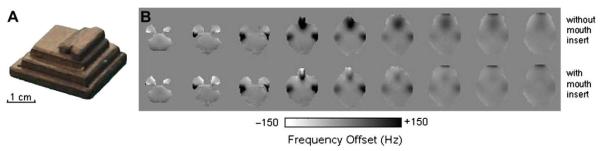
(A) Photograph of the highly-ordered pyrolytic graphite shim assembly. (B) Axial magnetic field maps without and with use of an intra-oral diamagnetic passive shim. Reproduced from [77] with permission of Wiley-Liss, Inc., a subsidiary of John Wiley and Sons, Inc.
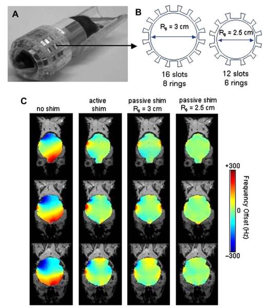
(A) Photograph of a combined diamagnetic and paramagnetic shim assembly on the mouse brain. (B) Shim former radii and shim element positioning for two prototyped constructions. (C) Field map (B0 = 9.4T) images demonstrating the utility of the passive shim system over three coronal slices in the mouse brain, spanning a range of 3 mm. Residual field maps are shown for no shimming, active RT shimming, passive shimming with prototypes of R0 = 3.0 cm and R0 = 2.5 cm. Reproduced from [82] with permission of Elsevier.
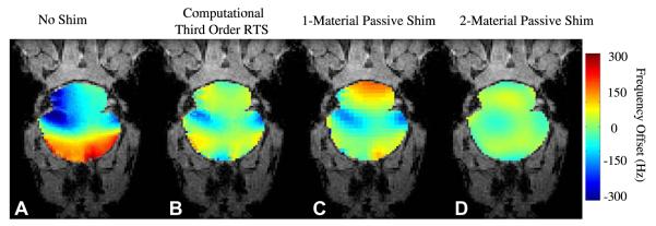
Reduction of higher-order inhomogeneity by active and passive shimming. Residual magnetic field maps (B0 = 9.4T) near auditory air cavities are presented using (A) no shim, (B) a computational third-order RTS, (C) computational one-material (zirconium) passive shim, and (D) computational two-material passive shim. Reproduced from [82] with permission of Elsevier.
Computed effects of volume parcellation on the global-homogenization capabilities of DSU. Anatomic images (A) and magnetic field maps at B0 = 3T are shown for three imaging planes using (B) static global shimming (96 × 96 × 96), whole-slice shimming (C) (96 × 96 × 1), and volume-parcellated shimming (D) (48 × 24 × 8). Results courtesy of Dr. Michael Poole.
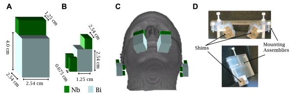
(A) Individual elements in sinus shim construction, (B) auditory shim construction (C) illustration showing full shim system, and (D) photographs of the shim construction.
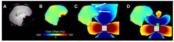
(A) sagittal anatomic gradient-echo MRI acquisition, (B) residual B0 inhomogeneity in the brain after whole-brain optimized first and second order RT shimming at B0 = 4T, (C) computed induction field and residual inhomogeneity using a local sinus passive shim as described in Fig. 22 without use of niobium, and (D) with use of niobium. Arrows indicate regions where unwanted effects are introduced by the non-shaped shim.
Field map assessment of passive-shim improvement over three axial slices (1–3) at B0 = 4T. (A) Gradient echo MRI, (B) residual inhomogeneity after zeroth through second order RT shimming, and (C) residual inhomogeneity after local passive shimming and zeroth through second-order RT shimming.

Gradient-echo images (B0 = 4T, TE = 35 ms, slice-thickness = 5 mm, oblique angle = 20°, 128 × 128 pixels over 24 cm × 19 cm) collected without (A) and with (B) local passive shims.
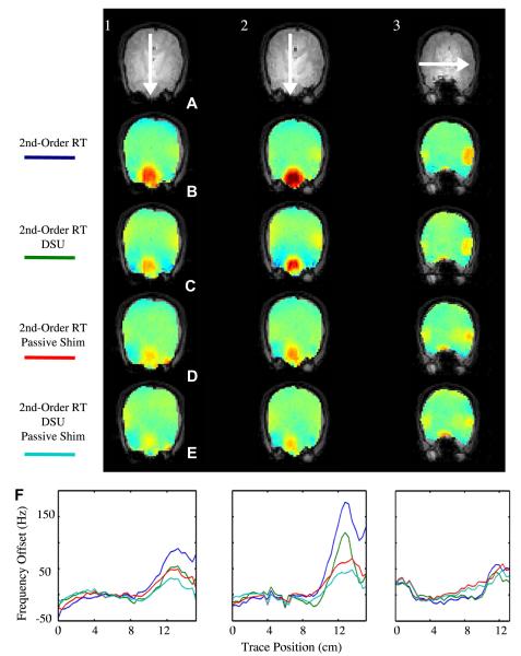
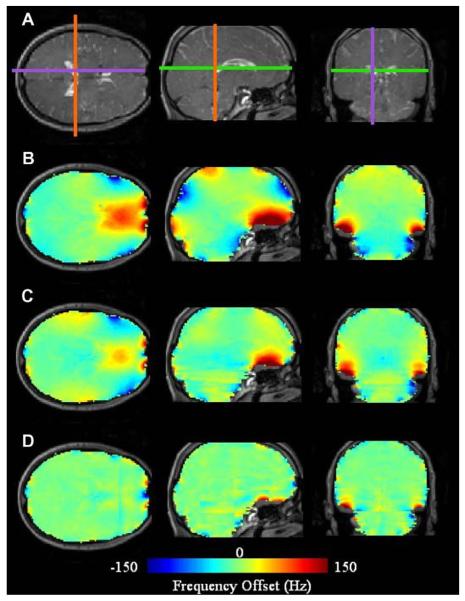
Field-mapping results with utility of combined DSU and passive shimming. Axial MRI images of three slices near the auditory and sinus cavities show the position of field map traces. Residual inhomogeneity after (A) zeroth through second-order RT shimming, (B) RT and DSU shimming, (C) RT and passive shimming, and (D) RT, DSU, and passive shimming. (D) Field-map traces as indicated in MRI (A). B0 = 4T. (For interpretation of color mentioned in this figure the reader is referred to the web version of the article.)
References
-
- Chen CN, Hoult DI. Biomedical Magnetic Resonance Technology. Adam Hilger; New York: 2005.
-
- Neuberth G. US Patent. 6,897,750 2005.
-
- Jackson JD. Classical Electrodynamics. John Wiley and Sons; New York: 1999.
-
- Salomir R, de Senneville BD, Moonen CTW. Concepts Magn. Reson. B. 2003;19:26–34.
-
- Marques JP, Bowtell R. Concepts Magn. Reson. B. 2005;25:65–78.
Grants and funding
LinkOut - more resources
Full Text Sources
Other Literature Sources
