Axonal velocity distributions in neural field equations

Abstract

By modelling the average activity of large neuronal populations, continuum mean field models (MFMs) have become an increasingly important theoretical tool for understanding the emergent activity of cortical tissue. In order to be computationally tractable, long-range propagation of activity in MFMs is often approximated with partial differential equations (PDEs). However, PDE approximations in current use correspond to underlying axonal velocity distributions incompatible with experimental measurements. In order to rectify this deficiency, we here introduce novel propagation PDEs that give rise to smooth unimodal distributions of axonal conduction velocities. We also argue that velocities estimated from fibre diameters in slice and from latency measurements, respectively, relate quite differently to such distributions, a significant point for any phenomenological description. Our PDEs are then successfully fit to fibre diameter data from human corpus callosum and rat subcortical white matter. This allows for the first time to simulate long-range conduction in the mammalian brain with realistic, convenient PDEs. Furthermore, the obtained results suggest that the propagation of activity in rat and human differs significantly beyond mere scaling. The dynamical consequences of our new formulation are investigated in the context of a well known neural field model. On the basis of Turing instability analyses, we conclude that pattern formation is more easily initiated using our more realistic propagator. By increasing characteristic conduction velocities, a smooth transition can occur from self-sustaining bulk oscillations to travelling waves of various wavelengths, which may influence axonal growth during development. Our analytic results are also corroborated numerically using simulations on a large spatial grid. Thus we provide here a comprehensive analysis of empirically constrained activity propagation in the context of MFMs, which will allow more realistic studies of mammalian brain activity in the future.

Figure 1. Dispersive propagator: synaptic connectivity and marginal velocity distribution.

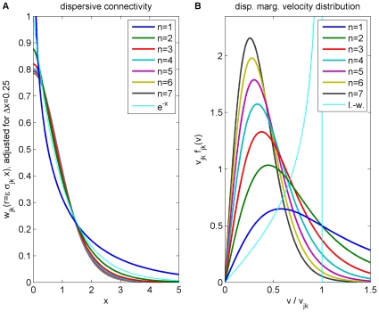
(A) Synaptic connectivity for different powers , which has been adjusted to match an exponential decay (thin curve). While the curves are continuous here, adjustment with Eq. (25) assumes a bin size , see text for details. (B) Marginal velocity distribution for different powers . Note that concerning the dimensionless ratio one obtains . The long-wavelength approximation of Eq. (36) is shown for comparison as thin curve. See Eqns. (19) and (32) for (A) and (B), respectively.

Figure 2. Cumulative distance-dependent velocity distributions: dispersive propagator vs. long-wavelength approximation.

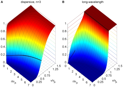
Shown are cumulative distributions integrated over as in Eq. (30). Dotted black lines on the base and on the plot surface show a grid of and values, solid black lines on the plot surface show the positions of the maxima of the unintegrated distributions. (A) Dispersive propagator for , where corresponds to Eqn. (28). (B) Long-wavelength approximation, where integrates Eqn. (33). We set and for comparison.

Figure 3. Difference propagator: synaptic connectivity and marginal velocity distribution.

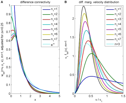
This figure is like Fig. 1, but for the difference propagator with . (A) Synaptic connectivity fit to an exponential decay (thin curve), Eqns. (47) and (49) are used. (B) Marginal velocity distribution Eq. (51). The dispersive case is shown as thin curve for comparison.

Figure 4. Confidence levels obtained from fits to the data in Tab. 2.

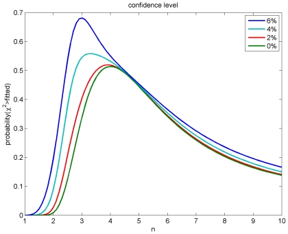
The power of Eq. (54) was varied in steps of 0.1 for four different uncertainties of the observed threshold diameters . The assumed relative diameter error reflects mainly differential shrinkage. As confidence level the probability that is greater than the fitted is shown.

Figure 5. Fits to threshold counts of myelinated fibre diameters in human corpus callosum.

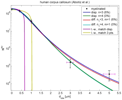
The diameter data is collected in Tab. 2, and the fit results with the dispersive Eq. (54) and difference Eq. (55) in Tab. 3. For the dispersive propagator the and fits are shown, which are optimal assuming equal to 6% and 0%, respectively. This relative diameter error (magenta error bars: 6%) reflects mainly differential shrinkage. Corresponding difference propagator fits are also shown, which have basically the same confidence levels. Thus these data cannot distinguish the dispersive and difference models, and the former is preferred for its computational simplicity. For the long-wavelength propagator a reasonable fit with Eq. (56) to all data cannot be obtained. Two curves are shown: one matching the median velocity of the dispersive case, the other fitting only the first three data points with .

Figure 6. Fits to binned counts of unmyelinated fibre diameters in rat subcortical white matter.

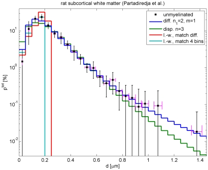
The binned diameter data are averages over the unmyelinated data shown in Figs. 4– 6 of Partadiredja et al. . (magenta error bars) has been assumed to reflect mostly differential shrinkage, but fit dependence on this is mild. Fit results using the difference Eq. (57), and its dispersive counterpart Eq. (58), are collected in Tab. 4. For unmyelinated axons the optimal fit with , is shown. For comparison, the optimal fit with the dispersive propagator is also displayed. It is viable, but has a three times larger . For the long-wavelength propagator a reasonable fit with Eq. (59) to all data cannot be obtained. Two curves are shown for illustration: one matching the median velocity of the difference , case, the other fitting only the first four data points.

Figure 7. Fits to binned counts of myelinated fibre diameters in rat subcortical white matter.

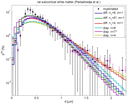
Data and fits are obtained as for Fig. 6, but using the myelinated counts. Two regular difference fit curves are shown: and , with in both cases. Systematic deviations from data around are obvious, but fit quality remains tolerable with a confidence level of 53.45% for . Even larger can increase the confidence level to about 70%. For comparison, dispersive fits with orders and are also shown. Their is almost a factor two larger, rendering their confidence level negligible. Fits with the long-wavelength propagator are not show, but fail drastically, cf. Fig. 6. The curves marked with a show additional fits for diameters only, i.e., without the first four data bins. Then one can find optimal fit orders for both propagators. These fits are of comparable, excellent quality compared to the reduced data set. But both predict too many small diameter fibres, and hence have negligible confidence levels compared to the full data set, with the dispersive again being about two times larger.

Figure 8. Comparison of combined marginal velocity distributions: human corpus callosum vs. rat subcortical white matter.

Shown are unmyelinated and myelinated contributions, and their sum: for human corpus callosum according to Eq. (61) and for rat subcortical white matter according to Eq. (62). The lower and upper borders of the bands are the minimum and maximum envelope, respectively, of all the “best fit” alternatives indicated in these equations, cf. Tab. 5. Since there is only one estimate for the human unmyelinated contribution, in that case a line instead of a band is drawn.

Figure 9. Turing instability analysis of the dispersive and long-wavelength propagators.

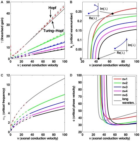
Bifurcations are investigated by varying the axonal conduction velocity and determining , , and the critical linearized gain . All other model parameters remain at the values discussed in the text. (A) Solid curves represent Turing-Hopf bifurcations (), dot-dashed curves Hopf bifurcations (). Results for orders of the dispersive propagator and for the long-wavelength model are shown. Above the Turing-Hopf curves travelling waves emerge, whereas above the Hopf curves bulk oscillations are seen. Stability will be lost at a given through the less stable bifurcation, which has smaller critical . (B) Critical wavenumber of the Turing-Hopf bifurcation. Insets show the position in the complex plane of the most weakly damped pole under variations of (open circles , closed circles ) for the dispersive model at the indicated . (C) Critical frequency of the less stable bifurcation. (D) Critical phase velocity , shown where Turing-Hopf is the less stable bifurcation.

Figure 10. Typical simulation result of the dispersive neural system far beyond a critical Turing-Hopf boundary.

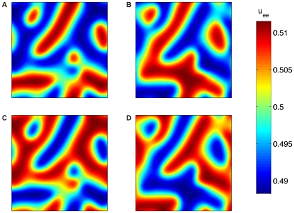
Subplots (A)–(D) represent successive snapshots of the spatial patterns of activity in spaced a quarter of the average temporal oscillation period apart. The dispersive propagator model of Eqns. (66)–(68) was computed for and with chosen well beyond the Turing-Hopf critical value, cf. Fig. 9A. Spatial derivatives were approximated using finite differences on a regular square grid of with spacing . The resulting system of equations was rewritten as a first-order system and integrated using ode45 in MATLAB starting from random initial conditions in . See also the supplementary Video S1 for the corresponding animation.

References

-
- Wilson HR, Cowan JD. A mathematical theory of the functional dynamics of cortical and thalamic nervous tissue. Kybernetik. 1973;13:55–80. - PubMed
- Lopes da Silva FH, Hoeks A, Smits H, Zetterberg LH. Model of brain rhythmic activity: The alpha-rhythm of the thalamus. Kybernetik. 1973;15:27–37. - PubMed
- Freeman WJ. Mass action in the nervous system: Examination of the neurophysiological basis of adaptive behavior through the EEG. New York: Academic Press, 1st edition; 1975. Cf. http://sulcus.berkeley.edu/MANSWWW/MANSWWW.html.
- Lopes da Silva FH, van Rotterdam A, Barts P, van Heusden E, Burr W. Models of neuronal populations: The basic mechanism of rhythmicity. Prog Brain Res. 1975;45:281–308. - PubMed
Publication types
MeSH terms
LinkOut - more resources
Full Text Sources