Global inhibition and stimulus competition in the owl optic tectum

Abstract

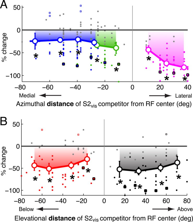
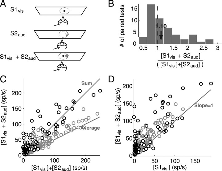
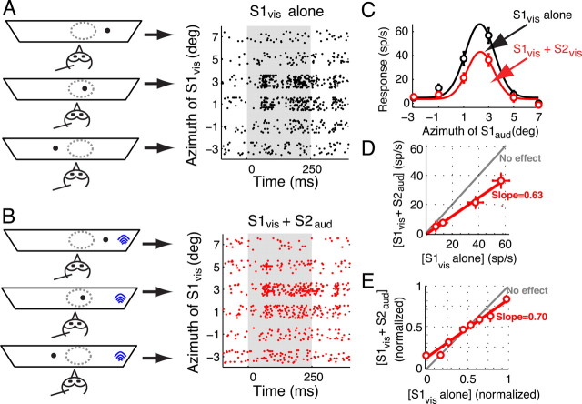
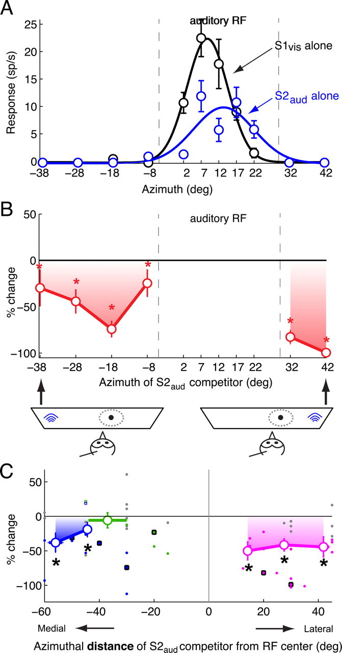
Stimulus selection for gaze and spatial attention involves competition among stimuli across sensory modalities and across all of space. We demonstrate that such cross-modal, global competition takes place in the intermediate and deep layers of the optic tectum, a structure known to be involved in gaze control and attention. A variety of either visual or auditory stimuli located anywhere outside of a neuron's receptive field (RF) were shown to suppress or completely eliminate responses to a visual stimulus located inside the RF in nitrous oxide sedated owls. The essential mechanism underlying this stimulus competition is global, divisive inhibition. Unlike the effect of the classical inhibitory surround, which decreases with distance from the RF center and shapes neuronal responses to individual stimuli, global inhibition acts across the entirety of space and modulates responses primarily in the context of multiple stimuli. Whereas the source of this global inhibition is as yet unknown, our data indicate that different networks mediate the classical surround and global inhibition. We hypothesize that this global, cross-modal inhibition, which acts automatically in a bottom-up manner even in sedated animals, is critical to the creation of a map of stimulus salience in the optic tectum.

Figure 1.

Neuronal responses to looming and stationary dots. A, Raster display of OTi-d neuronal responses to looming, black dots of different loom speeds. The duration of the stimulus, indicated by the gray box, was 0–250 ms. B, Raster display of responses of the same unit to stationary, black dots of different sizes (radii). The sizes tested correspond to the final dot sizes for each of the loom speeds tested in A. The duration of the stimulus, indicated by the gray box, was 0–250 ms. C, Neuronal responses to loom speed and dot size (black and blue circles, respectively, shown as mean ± SEM) obtained from A and B by counting spikes from 0 to 400 ms after stimulus onset and converting to spikes per second. The curves are difference of Gaussian models that fit best to the data (see Materials and Methods). Loom speeds and the corresponding final dot sizes are indicated along the x-axis. The maximum suppression (response at largest dot size or loom speed/peak response) in both curves is at the 10-percentile value of the respective distributions of maximum suppression (n = 19 sites). D, Total number of spikes (per second) in response to looming dots (black curve) and stationary dots (blue curve), calculated from a population of 19 sites at which both types of stimuli were tested. The error bars indicate the SE, estimated by applying a bootstrapping procedure with 1000 resamplings.

Figure 2.

Responses to paired looming visual stimuli inside the RF. A, Schematic representation of the experimental set-up showing (in top-view) an owl, a recording electrode, the tangent screen, the visual RF of the site (dotted circle). One visual stimulus (S1_vis, small black dot) was a looming stimulus presented at the RF center, and the second (S2_vis, larger black dot) was a faster looming visual stimulus presented inside the RF such that it did not physically overlap with S1_vis. B, Distribution of the ratio of responses to two looming visual stimuli (S1_vis and S2_vis) presented simultaneously inside the RF to the sum of the responses to each stimulus presented alone for all paired tests (n = 30 sites; 118 paired-stimulus tests). The properties of S1_vis and S2_vis are given in the text. C, Responses to the two looming visual stimuli presented simultaneously plotted against the sum of the responses to each stimulus alone. The data indicate mean values. The lines along which the data points would fall if the responses to S1_vis and S2_vis were equal to either the sum or the average of the individual responses are indicated. D, Responses to the two looming visual stimuli presented simultaneously plotted against the responses to S1_vis alone. The line along which the data points would fall if the responses to S1_vis and S2_vis were equal to the responses to S1_vis alone is indicated.

Figure 3.

Effect of a distant visual competitor on visual tuning curves. A, Left, Schematic representation of the experimental setup showing a single looming stimulus (black dot) at various locations. The arrows point to the responses obtained at each of the depicted stimulus configurations. Right, Raster display of neuronal responses to a single looming stimulus (S1_vis) presented at various azimuthal locations. Stimulus duration = 250 ms. Positive (negative) azimuthal values represent contralateral (ipsilateral) locations relative to the recording site. B, Left, Schematic representation of stimulus locations when two looming visual stimuli were presented. One stimulus (competitor, S2_vis, shown as a blue dot) was always far outside the RF (30° lateral) while another (S1_vis, shown as a black dot) traversed the RF in azimuth. Right, Raster display of the neuronal responses when both S1_vis and S2_vis were presented. Conventions as in A. C, Responses of the OTi-d site plotted as a function of the azimuth of the S1_vis stimulus when it was presented alone (black) or together with the S2_vis competitor (red). The data indicate mean ± SEM. The azimuthal tuning curves, obtained as the best-fit Gaussian to the responses in each condition, are also shown. D, Responses to the S1_vis and S2_vis stimuli presented together compared with the responses to the S1_vis stimulus alone. Responses to only those locations at which S1_vis was inside the RF (i.e., locations at which S1_vis elicited above-baseline activity; see Materials and Methods) are plotted. Linear regression of these responses yielded a fit with a slope of 0.57 that was significantly different from 1 (p < 0.05, Materials and Methods) and an intercept of −3.6 spikes/s that was not significantly different from 0 (p = 0.6). The gray line indicates no effect of the competitor stimulus. E, Population summary (n = 25 sites, 113 points). All responses at each site were normalized to the maximum response obtained at that site when S1_vis was presented alone. Data from all the sites were binned based on the values of the normalized responses to S1_vis alone (bin size 0.15) and plotted (mean ± SEM). Linear regression of these normalized and binned responses yielded a fit with a slope (1/divisive factor) of 0.50 (significantly different from 1, p < 0.05; see Materials and Methods), and a y-intercept (additive factor) of 7% (significantly different from 0, p = 0.02; see Materials and Methods).

Figure 4.

Spatial profile of the effect of a visual competitor on responses to a visual stimulus centered in the RF. A, Azimuthal tuning: responses and best-fit Gaussian profiles of an OTi-d site to single looming stimuli presented at different azimuths. S1_vis (loom speed = 8°/s, black) and S2_vis (speed = 14°/s, blue). Positive (negative) azimuths represent locations contralateral (ipsilateral) with respect to the recording site. The data indicate mean ± SEM. B, Elevational tuning: responses and best-fit Gaussian profiles for the same site as in A. Positive (negative) elevations represent locations above (below) the visual plane. C, Top, Azimuth-response profile for paired looming stimuli. Site exhibited a pronounced effect in the presence of S2_vis. Responses to S1_vis and S2_vis presented simultaneously as percentage changes (mean ± SEM) with respect to the responses to the S1_vis stimulus presented alone. S1_vis was presented at the RF center, while S2_vis was presented at various azimuths outside the RF. Asterisks indicate significant response suppression (p < 0.05, see Materials and Methods). Bottom, Schematic diagram showing the stimulus configuration for two extreme S2_vis locations. D, Top, Elevation-response profile for paired looming stimuli. Site exhibited a pronounced effect in the presence of S2_vis. Same conventions as in C.

Figure 5.

Population summary of the spatial profile of the effect of a visual competitor on responses to a visual stimulus centered in the RF. A, Summary of the effect of the azimuthal position of a looming visual stimulus (S2_vis) located outside the RF on responses to a weaker looming visual stimulus (S1_vis) presented near the RF center (n = 33). Responses are shown as percentage changes (mean ± SEM) with respect to the responses to S1_vis alone, and are plotted as a function of the azimuthal distance of S2_vis from the RF center. Only locations that were outside the RF (i.e., locations at which single stimuli did not drive responses; Materials and Methods) were included. Positive values of distance represent locations lateral to the RF center; negative values represent locations medial to the RF. Filled dots indicate data from individual sites; large open circles indicate the average effect (see Materials and Methods); gray dots indicate individual data that were not significantly different from 0 (see Materials and Methods); squares with black borders indicate the data from the example site in Figure 4. Locations lateral to the RF are shown in pink, those medial to the RF center and up to 15° into the opposite hemifield (represented on the same side of the brain) are shown in green, locations >15° into the opposite hemifield (represented on the opposite side of the brain) are shown in blue. Asterisks indicate significant response suppression (p < 0.05, see Materials and Methods). B, The effect of the elevational position of a looming visual stimulus (S2_vis) located outside the RF on responses to a weaker looming visual stimulus (S1_vis) presented near the RF center (n = 24). Same conventions as in A. Positive (negative) values of distance represent locations above (below) the RF center. Asterisks indicate significant response suppression (p < 0.05, see Materials and Methods).

Figure 6.

Responses to paired visual and auditory stimuli inside the RF. A, Schematic representation of the experimental set-up. S1_vis (small black dot) was a looming stimulus presented at the RF center, and S2_aud (black arcs) was an auditory stimulus presented inside the auditory RF. B, Distribution of the ratio of responses to a pair of visual (S1_vis) and auditory stimuli (S2_aud) presented simultaneously inside the RF to the sum of the responses to each stimulus presented alone for all paired tests (n = 14 sites; 69 paired-stimulus tests). The properties of S1_vis and S2_aud are given in the text. C, Responses to the paired visual (S1_vis) and auditory stimuli (S2_aud) plotted against the sum of the responses to each stimulus alone. The data indicate mean values. The lines along which the data points would fall if the responses to [S1_vis + S2_aud] were equal to either the sum or the average of the individual responses are indicated. Responses to two visual stimuli presented inside the visual RF (Fig. 2C) are reproduced for comparison (gray circles). D, Responses to the paired visual (S1_vis) and auditory stimuli (S2_aud) presented simultaneously plotted against the responses to S1_vis alone. The line along which the data points would fall if the responses to S1_vis and S2_aud were equal to the responses to S1_vis alone is indicated. Responses to two visual stimuli presented inside the visual RF (Fig. 2D) are reproduced for comparison (gray circles).

Figure 7.

Effect of a distant auditory competitor on visual tuning curves. A, Left, Schematic representation of the experimental set-up showing a single looming stimulus (black dot) at various locations. The arrows point to the responses obtained with each of the depicted stimulus configurations. Right, Raster display of neuronal responses to a single looming stimulus (S1_vis) presented at various azimuthal locations. Stimulus duration = 250 ms. Positive (negative) azimuthal values represent contralateral (ipsilateral) locations relative to the recording site. B, Left, Schematic representation of stimulus locations when visual and auditory stimuli were simultaneously presented. The auditory stimulus (competitor, S2_aud, shown as blue arcs) was always far outside the auditory RF (30° lateral) while the visual stimulus (S1_vis, shown as a black dot) traversed the visual RF in azimuth. Right, Raster display of the neuronal responses when both S1_vis and S2_aud were presented. Conventions as in A. C, Responses of an OTi-d site plotted as a function of the azimuth of a looming visual stimulus (S1_vis) presented alone (black), or together with a noise burst, auditory competitor (S2_aud; red). The auditory stimulus was located 30° lateral to the RF center. The properties of the stimuli are given in the text. The data indicate mean ± SEM. The azimuthal tuning curves, obtained as the best-fit Gaussian to the responses in each condition, are also shown. D, Responses to the S1_vis and S2_aud stimuli presented together compared with the responses to the S1_vis stimulus alone. Linear regression yielded a fit with a slope of 0.63 (significantly different from 1, p < 0.05; Materials and Methods) and an intercept that was not significantly different from 0. The gray line indicates no effect of the competitor stimulus. E, Population summary (n = 14 sites, 64 points). Responses to S1_vis presented along with S2_aud and responses to S1_vis alone are normalized, binned and plotted as described for Figure 3E. Linear regression of these normalized and binned responses yielded a fit with a slope (1/divisive factor) of 0.70 (significantly different from 1, p < 0.05; Materials and Methods), and a y-intercept (additive factor) of 13% in normalized coordinates (significantly different from 0, p = 0.005, see Materials and Methods).

Figure 8.

Spatial profile of the effect of an auditory competitor on responses to a looming visual stimulus centered in the RF. A, Azimuthal tuning: responses and best-fit Gaussian profiles of an OTi-d site to a single looming visual stimulus (S1_vis; loom speed = 8°/s, black) and a single noise burst auditory stimulus (S2_aud; 20 dB above threshold noise burst; blue). Positive (negative) azimuths represent locations contralateral (ipsilateral) with respect to the recording site. The data indicate mean ± SEM. B, Top, Azimuth-response profile for paired S1_vis and S2_aud stimuli. Site exhibited a pronounced effect in the presence of S2_aud. Responses to S1_vis and S2_aud presented simultaneously as percentage changes with respect to the responses to the S1_vis stimulus presented alone. S1_vis was presented near the RF center, while S2_aud was presented at various azimuths outside the auditory RF. Asterisks indicate significant response suppression (p < 0.05, see Materials and Methods). Bottom, Schematic diagram showing the stimulus configuration for two extreme S2_aud locations. C, Summary of the effect of the azimuthal position of an auditory stimulus (S2_aud) located outside the auditory RF on responses to a looming visual stimulus (S1_vis) presented near the RF center (n = 14). Responses are shown as percentage changes with respect to the responses to the S1_vis stimulus alone and are plotted as a function of the azimuthal distance of S2_aud from the RF center. Only locations that were outside the auditory RF (i.e., locations at which single auditory stimuli did not drive responses; see Materials and Methods) were included. Positive values of distance represent locations lateral to the RF center; negative values represent locations medial to the RF. Filled dots indicate data from individual sites; large open circles indicate the average effect (see Materials and Methods); gray dots indicate individual data that were not significantly different from 0 (see Materials and Methods); squares with black borders indicate the data from the example site in Figure 8B. Locations lateral to the RF are shown in pink, those medial to the RF center and up to 15° into the opposite hemifield (represented on the same side of the brain) are shown in green, locations >15° into the opposite hemifield (represented on the opposite side of the brain) are shown in blue. Asterisks indicate significant response suppression (p < 0.05, see Materials and Methods).

Figure 9.

Classical inhibitory surrounds of OTi-d neurons to stationary and looming dots. A, Excitatory (red) and inhibitory (blue) Gaussians obtained from a difference of Gaussians fit to the responses in Figure 1B, and the summed “Mexican hat” function (black). The radius of the local inhibitory surround for this unit estimated with stationary dots was 4.4°. B, Top, Raster display of unit responses to a looming stimulus of speed 20 deg/s (same site as in A and Fig. 1). Bottom, Mean and SEM of instantaneous firing rates from the raster (see Materials and Methods). The dashed arrow indicates firing rate at stimulus offset (r^off). *p < 0.05 (t test against 0). Gray, solid arrows indicate the peak firing rate and the time to peak rate. C, Pseudocolor plot of instantaneous firing rate at the same site for all tested values of loom speed. Green arrowhead corresponds to the loom speed in B. D, Plot of r^off as a function loom speed. In green is the r^off for a loom speed of 20 °/s, from (B, bottom panel). The steady-state value is shown in blue, and loom speed that evoked a response within 5% of the steady-state value is shown in red. The final dot radius at this loom speed is an estimate of the radius of the local inhibitory surround for a looming stimulus.

References

1. Akaike H. A new look at the statistical model identification. IEEE Trans Automat Contr. 1974;19:716–723.
1. Alvarado JC, Vaughan JW, Stanford TR, Stein BE. Multisensory versus unisensory integration: contrasting modes in the superior colliculus. J Neurophysiol. 2007;97:3193–3205. - PubMed
1. Baccus SA. Timing and computation in inner retinal circuitry. Annu Rev Physiol. 2007;69:271–290. - PubMed
1. Baddeley A. Working memory: looking back and looking forward. Nat Rev Neurosci. 2003;4:829–839. - PubMed
1. Basso MA, Wurtz RH. Modulation of neuronal activity by target uncertainty. Nature. 1997;389:66–69. - PubMed
Publication types
LinkOut - more resources