

Visualizing neuronal network connectivity with connectivity pattern tables
- PMID: 20140265
- PMCID: PMC2816167
- DOI: 10.3389/neuro.11.039.2009
Visualizing neuronal network connectivity with connectivity pattern tables
Abstract
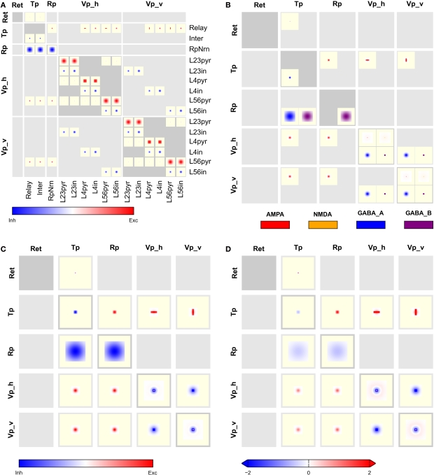
Complex ideas are best conveyed through well-designed illustrations. Up to now, computational neuroscientists have mostly relied on box-and-arrow diagrams of even complex neuronal networks, often using ad hoc notations with conflicting use of symbols from paper to paper. This significantly impedes the communication of ideas in neuronal network modeling. We present here Connectivity Pattern Tables (CPTs) as a clutter-free visualization of connectivity in large neuronal networks containing two-dimensional populations of neurons. CPTs can be generated automatically from the same script code used to create the actual network in the NEST simulator. Through aggregation, CPTs can be viewed at different levels, providing either full detail or summary information. We also provide the open source ConnPlotter tool as a means to create connectivity pattern tables.
Keywords: connectivity; neuronal network; population; projection; visualization.
Figures


Similar articles
-
Connectivity concepts in neuronal network modeling.PLoS Comput Biol. 2022 Sep 8;18(9):e1010086. doi: 10.1371/journal.pcbi.1010086. eCollection 2022 Sep. PLoS Comput Biol. 2022. PMID: 36074778 Free PMC article. Review.
-
Graffinity: Visualizing Connectivity in Large Graphs.Comput Graph Forum. 2017 Jun;36(3):251-260. doi: 10.1111/cgf.13184. Epub 2017 Jul 4. Comput Graph Forum. 2017. PMID: 29479126 Free PMC article.
-
PyNN: A Common Interface for Neuronal Network Simulators.Front Neuroinform. 2009 Jan 27;2:11. doi: 10.3389/neuro.11.011.2008. eCollection 2008. Front Neuroinform. 2009. PMID: 19194529 Free PMC article.
-
Efficient generation of connectivity in neuronal networks from simulator-independent descriptions.Front Neuroinform. 2014 Apr 22;8:43. doi: 10.3389/fninf.2014.00043. eCollection 2014. Front Neuroinform. 2014. PMID: 24795620 Free PMC article.
-
Engineering connectivity by multiscale micropatterning of individual populations of neurons.Biotechnol J. 2015 Feb;10(2):332-8. doi: 10.1002/biot.201400609. Epub 2015 Jan 13. Biotechnol J. 2015. PMID: 25512037
Cited by
-
BrainNet Viewer: a network visualization tool for human brain connectomics.PLoS One. 2013 Jul 4;8(7):e68910. doi: 10.1371/journal.pone.0068910. Print 2013. PLoS One. 2013. PMID: 23861951 Free PMC article.
-
ConGen-A Simulator-Agnostic Visual Language for Definition and Generation of Connectivity in Large and Multiscale Neural Networks.Front Neuroinform. 2022 Jan 7;15:766697. doi: 10.3389/fninf.2021.766697. eCollection 2021. Front Neuroinform. 2022. PMID: 35069166 Free PMC article.
-
VIOLA-A Multi-Purpose and Web-Based Visualization Tool for Neuronal-Network Simulation Output.Front Neuroinform. 2018 Nov 8;12:75. doi: 10.3389/fninf.2018.00075. eCollection 2018. Front Neuroinform. 2018. PMID: 30467469 Free PMC article.
-
Project, toolkit, and database of neuroinformatics ecosystem: A summary of previous studies on "Frontiers in Neuroinformatics".Front Neuroinform. 2022 Sep 26;16:902452. doi: 10.3389/fninf.2022.902452. eCollection 2022. Front Neuroinform. 2022. PMID: 36225654 Free PMC article. Review.
-
A federated design for a neurobiological simulation engine: the CBI federated software architecture.PLoS One. 2012;7(1):e28956. doi: 10.1371/journal.pone.0028956. Epub 2012 Jan 5. PLoS One. 2012. PMID: 22242154 Free PMC article.
References
-
- American Psychological Association. (2001). Publication Manual of the American Psychological Association. Washington, DC, American Psychological Association
-
- Austvoll K. (2007). Slicing Techniques for Hierarchical Neuronal Networks. Master's Thesis, Norwegian University of Life Sciences
-
- Austvoll K. (2009). Topology User Manual. NEST Initiative. http://www.nest-initiative.org/index.php/Software:Documentation
LinkOut - more resources
Full Text Sources