Noise and signal properties in PSF-based fully 3D PET image reconstruction: an experimental evaluation

Abstract

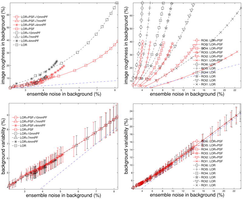
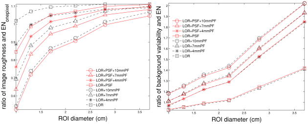
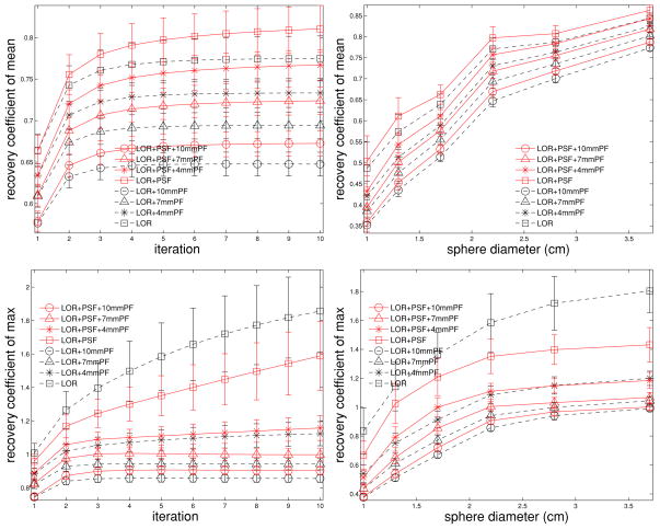
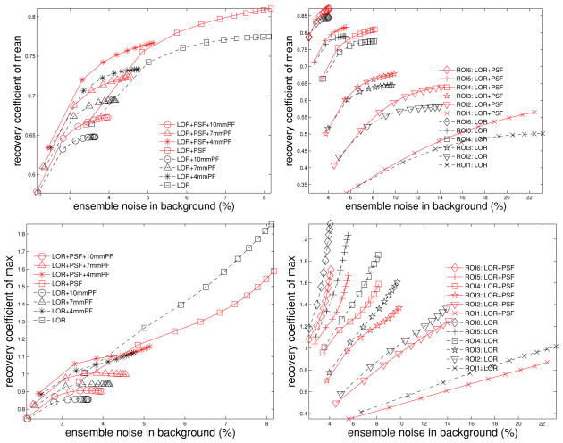
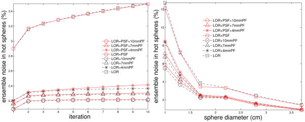
The addition of accurate system modeling in PET image reconstruction results in images with distinct noise texture and characteristics. In particular, the incorporation of point spread functions (PSF) into the system model has been shown to visually reduce image noise, but the noise properties have not been thoroughly studied. This work offers a systematic evaluation of noise and signal properties in different combinations of reconstruction methods and parameters. We evaluate two fully 3D PET reconstruction algorithms: (1) OSEM with exact scanner line of response modeled (OSEM+LOR), (2) OSEM with line of response and a measured point spread function incorporated (OSEM+LOR+PSF), in combination with the effects of four post-reconstruction filtering parameters and 1-10 iterations, representing a range of clinically acceptable settings. We used a modified NEMA image quality (IQ) phantom, which was filled with 68Ge and consisted of six hot spheres of different sizes with a target/background ratio of 4:1. The phantom was scanned 50 times in 3D mode on a clinical system to provide independent noise realizations. Data were reconstructed with OSEM+LOR and OSEM+LOR+PSF using different reconstruction parameters, and our implementations of the algorithms match the vendor's product algorithms. With access to multiple realizations, background noise characteristics were quantified with four metrics. Image roughness and the standard deviation image measured the pixel-to-pixel variation; background variability and ensemble noise quantified the region-to-region variation. Image roughness is the image noise perceived when viewing an individual image. At matched iterations, the addition of PSF leads to images with less noise defined as image roughness (reduced by 35% for unfiltered data) and as the standard deviation image, while it has no effect on background variability or ensemble noise. In terms of signal to noise performance, PSF-based reconstruction has a 7% improvement in contrast recovery at matched ensemble noise levels and 20% improvement of quantitation SNR in unfiltered data. In addition, the relations between different metrics are studied. A linear correlation is observed between background variability and ensemble noise for all different combinations of reconstruction methods and parameters, suggesting that background variability is a reasonable surrogate for ensemble noise when multiple realizations of scans are not available.

Figure 1

(a) Example of one transaxial slice of reconstructed image (using OSEM+LOR reconstruction without post-filtering, iteration = 5), with the black circle denoting the scanner field of view; (b) NEMA background ROIs (denoted by white spheres) overlaid on a zoomed transaxial slice.

Figure 2

Zoomed reconstructed images from one realization at iteration 2. Top: LOR; bottom: LOR+PSF. All images have the same color scale.

Figure 3

Zoomed reconstructed images from one realization at iteration 8. Top: LOR; bottom: LOR+PSF. All images have the same color scale.

Figure 4

Metrics for background noise. From top to bottom: image roughness, background variability, ensemble noise. Left column: noise metrics are plotted against iteration number with the ROI diameter fixed at 22 mm. Right column: noise metrics are plotted versus ROI size at fixed iteration 5. Error bars denote standard deviation across realizations.

Figure 5

Relations of noise metrics in background. From top to bottom: mean of image roughness (over realizations), and mean of background variability (over realization), plotted against the ensemble noise. Left column: relations of metrics are plotted with the ROI diameter fixed at 22 mm. Right column: relations of metrics are plotted for results without post-filtering. Error bars denote standard deviation across realizations, and the dash-dot line denotes the identity line.

Figure 6

The standard deviation image at iteration 5. Top: LOR; bottom: LOR+PSF. The ROI mean values of the background are shown above each corresponding image. All images have the same color scale.

Figure 7

Ratios of background noise metrics plotted versus ROI size at iteration 5. Left: ratio of image roughness and EN_onepixel. Right: ratio of background variability and ensemble noise.

Figure 8

Estimated background noise variance ${\sigma }_b^2$ (top) and average ROI noise covariance C̄ (bottom). Left column: metrics are plotted against iteration number with the ROI diameter fixed at 22 mm. Right column: metrics are plotted versus ROI size at fixed iteration 5.

Figure 9

Contrast recovery coefficient in hot spheres. From top to bottom: CRCmean, CRCmax. Left column: metrics are plotted against iteration number with the sphere diameter fixed at 22 mm. Right column: metrics are plotted versus sphere size at fixed iteration 5. Error bars denote standard deviation across realizations.

Figure 10

Relations of recovery coefficient in hot spheres and background noise. From top to bottom: mean of CRCmean (over realizations), and mean of CRCmax (over realizations), plotted against ensemble noise in background. Left column: relations of metrics are plotted with the sphere diameter fixed at 22 mm. Right column: relations of metrics are plotted for results without post-filtering.

Figure 11

Ensemble noise in hot spheres. Left: ensemble noise is plotted against iteration number with the sphere diameter fixed at 22 mm. Right: ensemble noise is plotted versus sphere size at fixed iteration 5.

Figure 12

SNR metrics of hot spheres. From top to bottom: SNRquant, SNRnpw. Left column: metrics are plotted against iteration number with the sphere diameter fixed (the sphere diameter is 22 mm for SNRquant, and 10 mm for SNRnpw). Right column: metrics are plotted versus sphere size at fixed iteration 5.

References

-
- Alessio AM, Kinahan PE, Harrison RL, Lewellen TK. IEEE Nucl. Sci. Symp. Conf. Record; Puerto Rico. 2005. pp. 1986–90.
- Alessio AM, Kinahan PE, Lewellen TK. IEEE Trans Med Imaging. 2006;25:828–37. - PubMed
- Barrett HH. J Opt Soc Am. 1990;7:1266–78. - PubMed
- Barrett HH, Wilson DW, Tsui BMW. Phys Med Biol. 1994;39:833–46. - PubMed
Publication types
MeSH terms
Grants and funding
LinkOut - more resources
Full Text Sources