Polymer gel dosimetry

Abstract

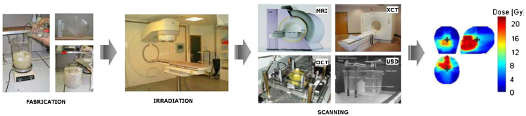
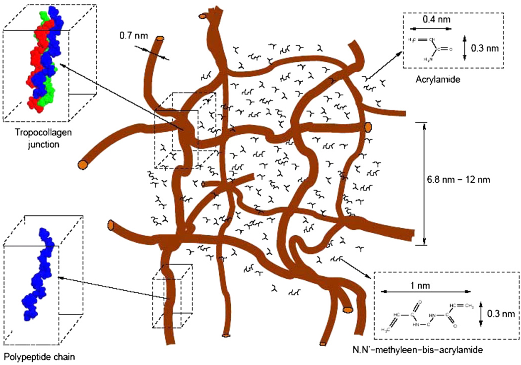
Polymer gel dosimeters are fabricated from radiation sensitive chemicals which, upon irradiation, polymerize as a function of the absorbed radiation dose. These gel dosimeters, with the capacity to uniquely record the radiation dose distribution in three-dimensions (3D), have specific advantages when compared to one-dimensional dosimeters, such as ion chambers, and two-dimensional dosimeters, such as film. These advantages are particularly significant in dosimetry situations where steep dose gradients exist such as in intensity-modulated radiation therapy (IMRT) and stereotactic radiosurgery. Polymer gel dosimeters also have specific advantages for brachytherapy dosimetry. Potential dosimetry applications include those for low-energy x-rays, high-linear energy transfer (LET) and proton therapy, radionuclide and boron capture neutron therapy dosimetries. These 3D dosimeters are radiologically soft-tissue equivalent with properties that may be modified depending on the application. The 3D radiation dose distribution in polymer gel dosimeters may be imaged using magnetic resonance imaging (MRI), optical-computerized tomography (optical-CT), x-ray CT or ultrasound. The fundamental science underpinning polymer gel dosimetry is reviewed along with the various evaluation techniques. Clinical dosimetry applications of polymer gel dosimetry are also presented.

Figure 1

Gel dosimetry involves three major steps in order to obtain a dose distribution: (a) after fabrication the gel is poured into an (antropomorphically shaped) cast and into calibration vials; (b) the phantom is irradiated with a specific dose distribution and calibration samples are irradiated to known doses; (c) the irradiated gel dosimeter phantoms are scanned with an appropriate and optimized scanning technique (magnetic resonance imaging (MRI), optical computerized tomography (optical-CT), x-ray computerized tomography (x-ray CT) or ultrasound; (d) finally the data are used to produce an image of the irradiated dose distribution.

Figure 2

Radiation-induced radiolysis of water by high-energy x-rays occurs in ‘spurs’ (a). The radiolytic products diffuse from the site of creation while recombination processes take place (De Deene 2004b). Reproduced with permission.

Figure 3

Consumption of AAm and Bis in a PAG as measured by Raman spectroscopy (Baldock et al 1998b). Reproduced with permission.

Figure 4

Dose–R2 response of both a (6%T/50%C) PAG and a corresponding AAm/Bis aqueous solution (APA). The dashed line corresponds to a spin–compartment model in the fast-exchange limit (Babic and Schreiner 2006). Reproduced with permission.

Figure 5

Representation of the microscopic structure of an unirradiated (6%T/50%C) polymer gel based on stoichiometric calculations.

Figure 6

Progression in polymer structure as a function of initial crosslinker concentration: (a) a gel solely composed of monomer (AAm). Long, linear chains are formed with no crosslinks; (b) gel composed of low initial Bis fraction. The predominant gel formation is an ordered, crosslinked network; (c) gel composed of high initial Bis fraction. Gels begin to form a larger number of knots; (d) a gel composed solely of crosslinker (Bis). The predominant structures are knots, loops and doublets which together form beads (Jirasek and Duzenli 2001b). Reproduced with permission.

Figure 7

Construction of an R2- and dose-images using a two points single spin–echo sequence (De Deene et al 1998b). Reproduced with permission.

Figure 8

Construction of R2- and dose-images using a multiple spin–echo sequence (De Deene et al 1998b). Reproduced with permission.

Figure 9

(a) Principle of magnetization transfer imaging. The polymer proton pool has a short T2 and thus covers a broader frequency line shape than the free water proton pool. By use of off-resonance saturation rf pulses part of the polymer protons is saturated. Because of magnetization transfer, polymer protons are exchanged with the water protons resulting in a decrease in longitudinal magnetization. (b) The observed relative signal decrease (MTR) is due to both direct saturation of the water protons (Mdir) and to magnetization transfer between the water proton pool and the polymer proton pool (MMT) (De Deene et al 2006a). Reproduced with permission.

Figure 10

(a) Dose response of a polymer gel, as derived from an imaging measurement (Wuu and Xu 2006); (b) Optical density of a polymer gel at a variety of doses, demonstrating the lack of absorption bands (Maryanski et al 1996). Reproduced with permission.

Figure 11

Schematic diagram of the different types of optical CT scanners: (a) first-generation laser system (Gore et al 1996); (b) fast laser scanner (Krstajic et al 2007); (c) cone-beam CCD scanner (Wolodzko et al 1999); (d) parallel-beam CCD scanner (Krstajic et al 2006). Reproduced with permission.

Figure 12

Examples of optical CT imaging using a laser system: (a) comparison of dose distributions in the central axial plane, with isodose lines at 40%, 60%, 100% and 115%, from treatment planning calculations (red), gel measurement (blue) and EDR2 measurements (green) (Wuu and Xu 2006); (b) same phantom as (a), results from sagittal plane 2 cm left of central plane. Reproduced with permission.

Figure 13

Examples of the effect of scatter in optical CT imaging: (a) square field image with diagonal cross artifact and (b) gamma map highlighting cross artifact (Islam et al 2003); (c) rendered optical CT image of a ‘funnel phantom’ and (d) profiles of reconstructed optical density across funnel phantom, showing both under- and over-estimation of the parameter (Bosi et al 2007, 2009b). Reproduced with permission.

Figure 14

(a) X-ray CT images of PAG irradiated with four 3 × 3 cm² 10 MV photon beams (doses in Gy at the depth of maximum dose) (a)–(c) and parallel opposed, 2 cm diameter, circular 6 MV photon beams (d). A preliminary CT image is shown in (a) and a noise reduced (by averaging) CT image in (b). Note the ring and beam hardening artifacts in (b). Images in (c) and (d) are the optimized images resulting from image averaging and background subtraction with the images acquired from an unirradiated blank gel. The dose profile along the axis of the 6 Gy beam path corresponding to the dose image of (c) is shown in (e) in comparison with a profile obtained in an MR acquired dose image (Hilts et al 2000). Reproduced with permission.

Figure 15

(a) Density of PAG as a function of dose. (b) Linear attenuation coefficient (μ) of PAG as a function of density (Trapp et al 2002). Reproduced with permission.

Figure 16

Adapative mean filtering (K = 11, n = 2) for synthetic ‘gel’ image (conformal prostate). (a) Noise free image with filtered image contour overlay, (b) profiles through noise-free, filtered and unfiltered images, and (c) dose area histograms of noise-free, filtered and unfiltered images (Hilts and Jirasek 2008). Reproduced with permission.

Figure 17

(a) Ultrasound tomography system. Transmission (b) and time-of-flight image (c) of a PAG irradiated with a 4 × 4 cm² square photon beam. Scan lines are acquired at a translational resolution of 1 mm and a rotational resolution of 2° with a total rotation of 360°. The reconstructed image resolution was 1.45 × 1.45 mm² (Mather and Baldock 2003). Reproduced with permission.

Figure 18

Gel dosimetry is performed in different stages. At each stage errors can add, leading to a decrease in the overall precision and accuracy (De Deene 2006). Reproduced with permission.

Figure 19

The calibration contribution factor (CCF) as a function of dose for various numbers of calibration points (N_cal). The values on the abscissa are relative to the maximum dose D_max in the calibration plot (De Deene et al 1998b). Reproduced with permission.

Figure 20

Schematic representation of an ideal voxel shape without any outer voxel contribution (left) and an actual voxel with spread of signal to neighboring voxels.

Figure 21

B1 field map (effective flip angle) acquired with the body coil (a) and with the head coil (d). R2 images of a blank unirradiated polymer gel dosimeter acquired with the body coil and head coil are shown in (c) and (f) showing the effect of the inhomogeneous B1 field for the head coil. The field-of-view (FOV) is 320 × 320 mm². Corresponding longitudinal profiles through the center are also shown (b and e). The plot in figure (g) gives the relation between the change in R2 and the flip angle for a nominal flip angle of 90° (De Deene et al 2000b). Reproduced with permission.

Figure 22

(a) Top-down model of dosimetric quality assurance (QA) in intensity-modulated radiotherapy. In the conceptual pyramid, each level of QA is based on the stability of the underlying levels. The two lower levels can be part of period equipment QA. For QA of a clinical class solution, one may start at the top by applying 3D dosimetry of an entire treatment. One descends the pyramid to the lower levels if the 3D dosimetry reveals intolerable discrepancies with treatment planning. (b) Methodology and tools appropriate for each of the levels. EPID stands for ‘electronic portal imaging’ (De Wagter et al 2004). Reproduced with permission.

Figure 23

(a) Stack of corresponding dose maps obtained by three different dosimetry techniques: gel dosimetry, film dosimetry and computer planning. (b) Color-washed difference images superimposed onto anatomical CT-images. (c) Mean structural root-mean-square difference (closed symbols) and stochastic root-mean-square difference (open symbols) in corresponding dose maps obtained with gel dosimetry and film dosimetry (De Deene et al 2000c). Reproduced with permission.

Figure 24

Dose verification of an IMAT treatment using polymer gel dosimetry. (a) A 10 l Barex cast was filled with PAG. At each side of the phantom, three slices of the anthropomorphic Rando phantom were added in the cranio-caudal direction to obtain full scatter conditions. Dose distributions in the middle transverse plane of the phantom as calculated with a collapsed cone convolution/superposition algorithm (b) and measured with polymer gel dosimetry (c). Corresponding dose–volume histograms for PTV, liver and kidneys are also shown (d) (Duthoy et al 2003). Reproduced with permission.

Figure 25

(a) PAG irradiated after irradiation with a source consisting of a train of 16 90Sr/90Y pellets inserted in glass (left) and Barex tubes (right). (b) Axial R2 image with an in-plane resolution of 0.2 mm. (c) Relative dose profiles obtained with polymer gel dosimetry and two different radiochromic films. (d) The longitudinal R2 image (Amin et al 2003). Reproduced with permission.

Figure 26

The variation in LET as a function of depth for a 133 MeV proton beam (dashed curve, left-hand side) and the measured relative sensitivity normalized to the measured dose at a depth of 60 mm (solid curve, right-hand side). Also shown is the corresponding depth–dose curve normalized to 100% at the Bragg peak (Gustavsson et al 2004). Reproduced with permission.

Figure 27

(a) Neutron irradiation setup: the epithermal neutron beam is incident from the left through a circular beam aperture (A); cylindrical gel phantom (B) is inserted into a cylindrical extension (C) of the water phantom (D); (b) calculated (solid line) and measured (dashed line) isodoses (10% intervals, starting from the 90% isodose) in the central cross-section of the cylindrical gel phantom. Also shown are two axial cross-sections (Uusi-Simola et al 2007).

Figure 28

(a) Water phantom with a normoxic polymer gel dosimeter centrally positioned for diagnostic CT-dose profiles and CTDI determination; (b) normoxic polymer gel dosimeter phantoms; (c) corresponding R2 image after exposure to x-rays from a CT scanner. The accumulated dose is from 50 accumulated single transaxial CT slices for 8 and 5 2020 mm slice widths (140 kVp, 400 mAs) (Hill et al 2005b). Reproduced with permission.

References

1. Adamovics J, Maryanski MJ. Characterisation of PRESAGE: a new 3-D radiochromic solid polymer dosemeter for ionising radiation. Radiat. Prot. Dosim. 2006;120:107–112. - PubMed
1. Alexander P, Charlesby A, Ross M. The degradation of solid polymethylmethacrylate by ionizing radiations. Proc. R. Soc. A. 1954;223:392.
1. Amin MN, Horsfield MA, Bonnett DE, Dunn MJ, Poulton M, Harding PF. A comparison of polyacrylamide gels and radiochromic film for source measurements in intravascular brachytherapy. Br. J. Radiol. 2003;76:824–831. - PubMed
1. Andrews HL, Murphy RE, LeBrun EJ. Gel dosimeter for depth dose measurements. Rev. Sci. Instrum. 1957;28:329–332.
1. Audet C, Hilts M, Jirasek A, Duzenli C. CT gel dosimetry technique: comparison of a planned and measured 3D stereotactic dose volume. J. Appl. Clin. Med. Phys. 2002;3:110–118. - PMC - PubMed