Efficient spatiotemporal analysis of the flagellar waveform of Chlamydomonas reinhardtii

Abstract

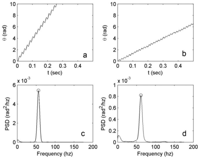
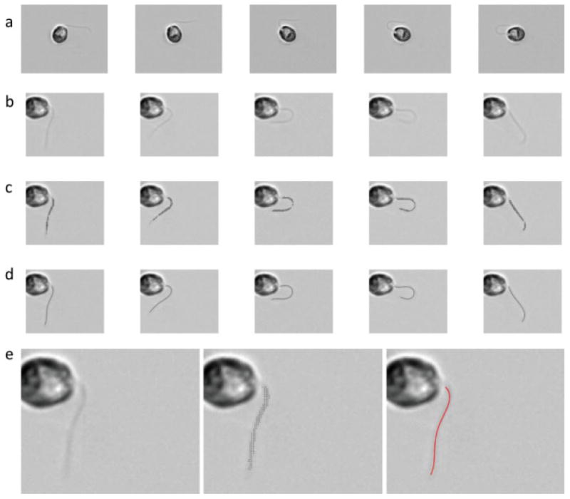
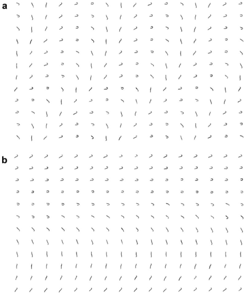
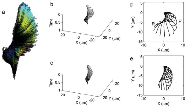
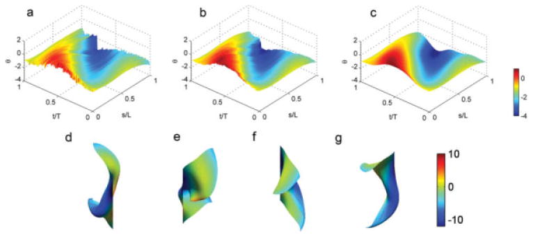
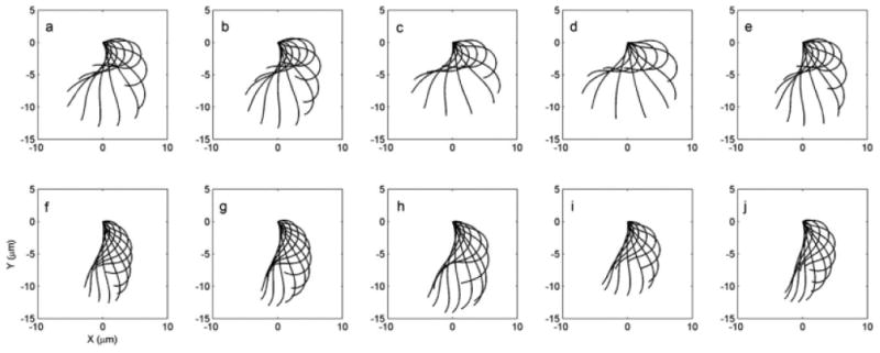
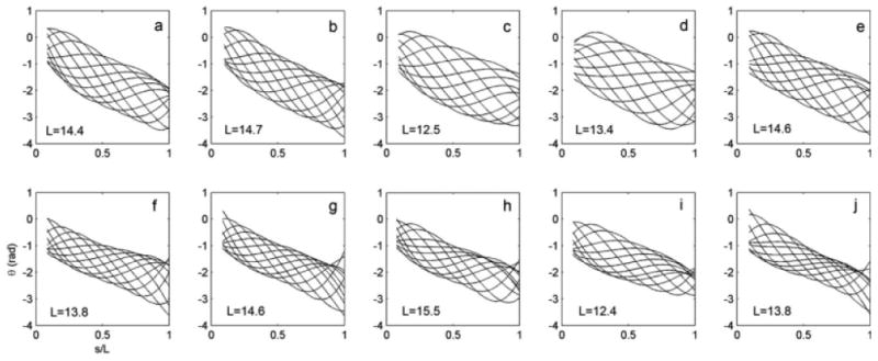
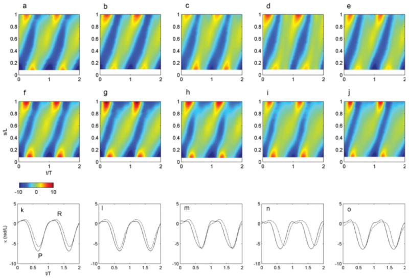
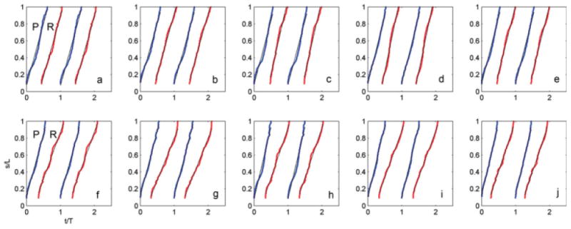
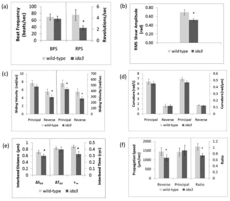
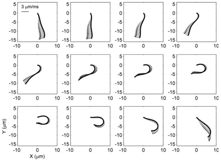
The 9 + 2 axoneme is a microtubule-based machine that powers the oscillatory beating of cilia and flagella. Its highly regulated movement is essential for the normal function of many organs; ciliopathies cause congenital defects, chronic respiratory tract infections and infertility. We present an efficient method to obtain a quantitative description of flagellar motion, with high spatial and temporal resolution, from high speed video recording of bright field images. This highly automated technique provides the shape, shear angle, curvature, and bend propagation speeds along the length of the flagellum, with approximately 200 temporal samples per beat. We compared the waveforms of uniflagellated wild-type and ida3 mutant cells, which lack the I1 inner dynein complex. Video images were captured at 350 fps. Rigid-body motion was eliminated by fast Fourier transform (FFT)-based registration, and the Cartesian (x-y) coordinates of points on the flagellum were identified. These x-y "point clouds" were embedded in two data dimensions using Isomap, a nonlinear dimension reduction method, and sorted by phase in the flagellar cycle. A smooth surface was fitted to the sorted point clouds, which provides high-resolution estimates of shear angle and curvature. Wild-type and ida3 cells exhibit large differences in shear amplitude, but similar maximum and minimum curvature values. In ida3 cells, the reverse bend begins earlier and travels more slowly relative to the principal bend, than in wild-type cells. The regulation of flagellar movement must involve I1 dynein in a manner consistent with these results.

Fig. 1

(a) Angle of rigid body rotation observed in a video of wild-type uni1-2 Chlamydomonas. Mean rotation rate is 6.13 revolutions per second. (b) Angle of rigid body rotation observed in a video of an ida3 mutant cell. Mean rotation rate is 2.08 revolutions per second. (c) Power spectral density function (PSD) of the oscillations in (a); the peak at 56.6 Hz represents the beat frequency of this wild-type cell. (d) Power spectral density function (PSD) of the oscillations in Fig. 2b, showing a beat frequency of 61.5 Hz for this ida3 cell.

Fig. 2. Overview of video analysis

(a) Video frames after the image background has been subtracted. (b) Video images after rigid-body motion has been removed. (c) “Point clouds” of pixels identified as belonging to the flagellum, superimposed on the video frames. (d) Curves obtained from fitting of a polynomial function (Eq. 1) to the point clouds shown above. Curve fitting was done after the sorting procedure described in the text and illustrated in Fig. 3. (e) Enlarged views of the first images in rows (b–d).

Fig. 3. Sorting of flagellar point clouds

(a) Unsorted point clouds. (b) Point clouds after sorting by order of phase in flagellar cycle, as identified by isometric feature mapping (Isomap). The first six rows of the sorted beat correspond to “recovery” as the primary bend propagates from base to tip; the last six rows roughly correspond to the “power stroke” driven by propagation of the reverse bend.

Fig. 4

(a) Point clouds sorted and plotted on x–y-time coordinate axes, along with the smoothed surface of Cartesian coordinates obtained by the fitting procedure. (b,c) Line plots showing the waveforms for wild-type and ida3 respectively in 3D (x–y-time coordinates). (d,e) Successive “snapshots” of the flagellar waveforms in 2D (x–y coordinates) of wild-type and ida3 respectively. In (d,e), for clarity waveforms are shown only at intervals of 1/12 cycle. P indicates the “primary” bend as it approaches the end of the flagellum; R indicates the “reverse” bend.

Fig. 5. (a–c) Surfaces of shear angle θ(s,t) as a function of distance along the flagellum, s, and time throughout the cycle

Distances are normalized by flagellar length, L, and time is normalized by the beat period, T. (a) An example surface constructed from unfiltered polynomial curves fitted to 200 point clouds. (b) The same surface after median filtering in time. (c) The same surface after median filtering and smoothing with gridfit; color represents shear angle. (d–g) Four different views of the Cartesian (x–y-time) surface corresponding to the smoothed θ(s,t) surface; color represents surface curvature.

Fig. 6. Waveforms from five representative videos of wild-type (a–e) and ida3 mutant cells (f–j)

For clarity, waveforms are shown only every 1/12 of a cycle.

Fig. 7. Shear angle θ plotted versus normalized distance along the flagellum for five representative videos of wild-type (a–e) and five ida3 cells (f-j)

Shear angle plots are shown at intervals of 1/12 cycle, corresponding to the waveforms of Fig. 6. Lengths (μm) are noted on each plot. Plots start at nonzero values of s/L because the flagellum cannot be well resolved within ∼ 1 μm of the proximal end.

Fig. 8. Curvature κ=dθds (normalized by flagellar length) plotted versus normalized time (t/T, horizontal axis) during the cycle and normalized distance along the flagellum (s/L, vertical axis), for five representative videos of wild-type (a–e) and ida3 cells (f–j)

(k–o) Plots of curvature versus time at the midpoint of the flagellum, showing that the duration of high negative curvature is shorter in ida3 flagella (dashed) than in wild-type flagella (solid), although minimum curvature values are similar. Each pair of curves corresponds to the two maps above them. These maps and plots correspond to the waveforms of Fig. 6; note that two beat cycles are shown.

Fig. 9. Time-space trajectories of the points of maximum and minimum curvature for the flagellar waveforms of Figs. 6–8

Top row: wild-type. The average ratio between the propagation speed of the reverse bend (slope of red line, R) and the propagation speed of the principal bend (slope of the blue curve, P) is 1.03 ± 0.09 (N = 12 wild-type cells). Bottom row: ida3. The average ratio between the propagation speed of the reverse bend and the propagation speed of the principal bend is 0.73 ± 0.09 (N = 12 ida3).

Fig. 10. Statistical comparison of the uni1 wild-type and ida3 flagellar waveforms

(a) Beat frequency (BPS = beats/s) and rotation rate (RPS = revs/s). (b) The average root-mean-square (RMS) amplitude of shear angle variation. (c) Sliding velocity measured in both nondimensional (rad/cyc) and physical units (rad/s). (d) Average values of the principal bend curvature and reverse bend curvature measured in both nondimensional (rad/length) and physical units (rad/μm). (e) Spatial and temporal measures of coordination between bends. The mean inter-bend distance ΔS_AV represents the average normalized distance between the points of minimum (principal) and maximum (reverse) curvature. The mean inter-bend time ΔT_AV represents the average time between the occurrence of the minimum (principal) and maximum (reverse) curvatures. The time delay τ_PR represents the delay between the initiation of the principal and the reverse bend. (f) Propagation speeds of the principal and reverse bends, and the ratio of propagation speeds (reverse/principal). In all summary plots, averages are computed over all time points and all locations in the middle 80% of the flagellum, and include all wild-type or ida3 cells.

Fig. 11. Velocity vectors at selected points on the flagellum at 12 equally-spaced times in the flagellar cycle (wild-type)

The enhanced spatial and temporal resolution provided by the current algorithm enables accurate estimation of velocity field. Other mechanical parameters, such as propulsive force and power can be estimated from the velocity field.

References

1. Bower R, VanderWaal K, O'Toole E, Fox L, Perrone C, Mueller J, Wirschell M, Kamiya R, Sale WS, Porter ME. IC138 defines a sub-domain at the base of the I1 dynein that regulates microtubule sliding and flagellar motility. Mol Biol Cell. 2009;20:3055–3063. - PMC - PubMed
1. Brokaw C. Automated methods for estimation of sperm flagellar bending parameters. Cell Motil Cytoskeleton. 1984;4:417–430. - PubMed
1. Brokaw C. Control of flagellar bending: a new agenda based on dynein diversity. Cell Motil Cytoskeleton. 1994;28:199–204. - PubMed
1. Brokaw C, Kamyia R. Bending patterns of Chlamydomonas flagella IV: mutants with defects in inner and outer dynein arms indicate differences in dynein arm function. Cell Motil Cytoskeleton. 1987;8:68–75. - PubMed
1. Brokaw C, Luck D. Bending patterns of Chlamydomonas flagella I: wild-type bending patterns. Cell Motil Cytoskeleton. 1983;3:131–150. - PubMed
Publication types
LinkOut - more resources