. 2010 Feb 24:11:106.
doi: 10.1186/1471-2105-11-106.

SpectraClassifier 1.0: a user friendly, automated MRS-based classifier-development system

Affiliations

SpectraClassifier 1.0: a user friendly, automated MRS-based classifier-development system

Sandra Ortega-Martorell et al. BMC Bioinformatics. .

Abstract

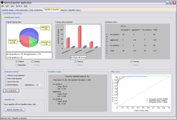
Background: SpectraClassifier (SC) is a Java solution for designing and implementing Magnetic Resonance Spectroscopy (MRS)-based classifiers. The main goal of SC is to allow users with minimum background knowledge of multivariate statistics to perform a fully automated pattern recognition analysis. SC incorporates feature selection (greedy stepwise approach, either forward or backward), and feature extraction (PCA). Fisher Linear Discriminant Analysis is the method of choice for classification. Classifier evaluation is performed through various methods: display of the confusion matrix of the training and testing datasets; K-fold cross-validation, leave-one-out and bootstrapping as well as Receiver Operating Characteristic (ROC) curves.

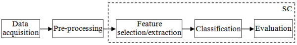
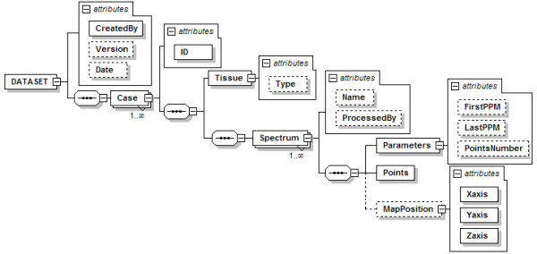
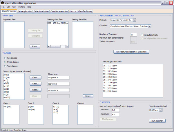
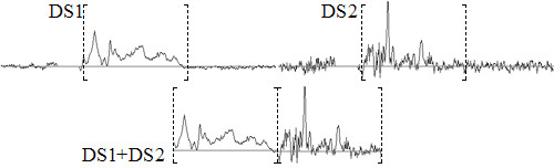
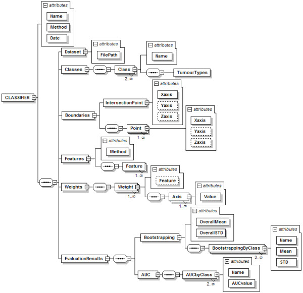
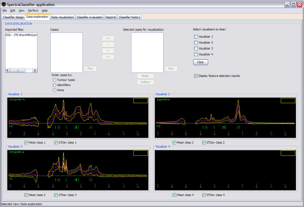
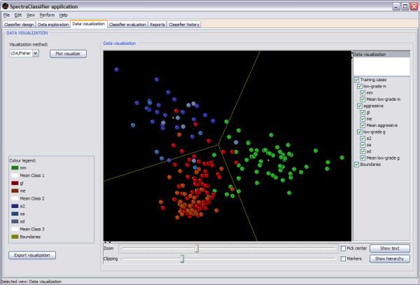
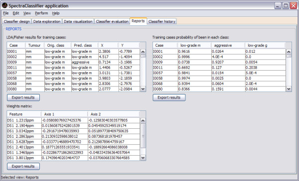
Results: SC is composed of the following modules: Classifier design, Data exploration, Data visualisation, Classifier evaluation, Reports, and Classifier history. It is able to read low resolution in-vivo MRS (single-voxel and multi-voxel) and high resolution tissue MRS (HRMAS), processed with existing tools (jMRUI, INTERPRET, 3DiCSI or TopSpin). In addition, to facilitate exchanging data between applications, a standard format capable of storing all the information needed for a dataset was developed. Each functionality of SC has been specifically validated with real data with the purpose of bug-testing and methods validation. Data from the INTERPRET project was used.

Conclusions: SC is a user-friendly software designed to fulfil the needs of potential users in the MRS community. It accepts all kinds of pre-processed MRS data types and classifies them semi-automatically, allowing spectroscopists to concentrate on interpretation of results with the use of its visualisation tools.


Figures

Figure 1
Figure 1
Steps covered by SC in a pattern recognition system. Most pattern recognition systems can be partitioned into these steps: data acquisition, which in our case obtains either the SV, MV or high resolution MRS data; pre-processing, which converts the raw data in the time domain into processed spectra in the frequency domain with the preferred pre-processing routines and protocols of choice; feature selection/extraction, to measure data vectors properties that are useful for classification; the classification, that uses these features to assign the data vector analysed to a category; and the evaluation, which assesses the model created. SC performs the last three steps (dotted box).
Figure 2
Figure 2
Flow chart representing the construction and validation of a classifier using SC. For developing a classifier using SC, the user can start by defining the training datasets, and then can follow this flow chart to develop a reliable and validated model.
Figure 3
Figure 3
Structure of the DATASET node. The global node is DATASET, and is composed by one or more Case nodes. A Case node has an ID attribute for the identification of the case, and a sequence of nodes: first the Tissue node, with a Type attribute for the tumour type; and then a sequence of one or more Spectrum nodes. Every Spectrum node has three child nodes: Parameters, Points, and MapPosition. The Points node is used to store the spectral quantitative data, i.e. the intensity value of each point in the frequency domain, and the MapPosition node is used to store the x-y position of each spectrum in each MV grid. Dashed lines are used to indicate non-mandatory elements.
Figure 4
Figure 4
Classifier design tab. The training data are imported into the "DATA SETS" frame. The "Imported files" can be assigned to either "Training data files" or to "Testing data files" by clicking on the respective buttons. The "CLASSES" frame allows selecting and combining cases to be used for the classifier as training and to establish their name and composition. On "Class name", one can write down the name of the desired class. "Tumour types (number of cases)" displays the number of cases of each type in the training dataset, which can be assigned to the preferred class for classification. Several types already set in the "Training data files" can be merged into the same classification class, therefore allowing different combinations of training data types, for hypothesis testing. The "FEATURE SELECTION AND EXTRACTION" frame allows choosing the desired feature selection or extraction technique and the evaluation method. In this example the "Sequential Forward FS" and "Correlation-based Feature Subset Selection" have been chosen. Clicking on the "Run Feature Selection or Extraction" button below gives the resulting features. "DS1" means "Dataset one", since it is possible to concatenate two spectra from the same case obtained under different acquisition conditions and therefore the first one entered would be DS1. The "CLASSIFIER" frame allows the user to choose the spectral range (in ppm) which will be the desired region of interest for feature selection or extraction and for classification. The "Run classifier" button allows starting the classification with the selected "Classification method" (currently, Fisher LDA).
Figure 5
Figure 5
Using two spectra by case. When using two spectra by case (for instance when having two acquisitions at two different TEs) the new spectrum will be formed concatenating the range of interest (bracketed intervals) of both spectra.
Figure 6
Figure 6
Structure of the CLASSIFIER node. The CLASSIFIER node has attributes for naming the classifier, indicating the classification method and the creation date; and it is composed by a sequence of six nodes: Dataset, Classes, Boundaries, Features, Weights, and EvaluationResults. The Dataset node has only the path to the dataset file. The Classes node contains a series of Class nodes for storing the tumour types involved in each class. The Boundaries node is for storing the points that form the boundaries between classes in the projection space: they are the intersection point (IntersectionPoint node) and the rest of points (the Point node sequence) used to draw a line from each of them to the intersection point. The Features node has the attribute Method for the name of the FS/FE method used, and the list of the resulting features. The Weights node contains the sequence of weights of the classifier, and the associated feature to each of them. The EvaluationResults node is for storing information related with the evaluation of the model, in this case, using bootstrapping (the Bootstrapping node) and the ROC curve (the AUC node). The Bootstrapping node has two attributes for the overall mean and standard deviation, and a list of nodes with the bootstrapping results per class. The AUC node contains a sequence of nodes with the AUC results by class. Dashed lines are used to indicate non-mandatory elements.
Figure 7
Figure 7
Data exploration tab. Continuing the example introduced in Figure 4, three of the four visualisers are showing the feature selection results: the mean (pink spectrum), the standard deviation range (yellow line) and the selected features (green vertical lines). Each visualiser displays the information of one class. The name of the class is written on the top left of the visualiser.
Figure 8
Figure 8
Data visualisation tab. Continuing the example of Figure 4, the projection space of the Fisher LDA classifier can be seen: low-grade m (mm, in green), aggressive (gl+me, in shades of red) and low-grade g (a2+oa+od, in shades of blue). This visualisation is a two-dimensional representation of the corresponding point in the space of each case, taking advantage of this visualisation by rotating it and twisting it around (using the mouse and the controls at the bottom of the visualisation panel), turning on or off parts of the display (using the check buttons components in the right of the visualiser), and identifying cases by selecting them with the mouse. As this example is a three-class classifier, a 2D display with the boundaries of the classes (yellow lines) is displayed.
Figure 9
Figure 9
Classifier evaluation tab. In this example (started in Figure 4), the top left graph is a pie plot that can be used to check the global information of the number of cases that originally belong to each class, and the number of cases that the classifier predicted to belong to each class. The top centre graph is a bar plot used for checking the numerical relationship between rightly (the red ones) and wrongly (the blue ones) predicted cases per class. The top right panel is a confusion matrix, useful for checking predicted cases in each class. For example: the low-grade m class actually contains 58 cases, but the classifier predicts 52 of them as low-grade m, the other 6 are predicted to be aggressive (5) and low-grade g (1). The confusion matrix can also be generated for an independent test set, improving the capabilities of the evaluation. The bottom centre panel shows the bootstrapping results for N = 1000 (a total mean accuracy of 91.28%, with a standard deviation of 1.846%). The bottom right graph is the ROC curve (in the case of a classifier with more than two classes, like the one on this example, data are analysed by dichotomisation [32]), showing the plot of a ROC curve and the AUC value per class.
Figure 10
Figure 10
Reports tab. In this example three reports are shown. On the top left of this tab the Fisher LDA results for training cases are shown: each row of the table corresponds to one case, showing its identifier, the tumour types, the actual original class, the predicted class (obtained by the Fisher LDA method), and the corresponding X and Y coordinates for the representation in a projection space. On the top right the Fisher LDA probabilities results for training and testing cases are shown: each row of the table corresponds to one case, showing its identifier and the probabilities of belonging to each previously defined class (low-grade m, aggressive, low-grade g). In the bottom left there is the weights matrix report, showing the matrix of weights of the classifier, each of them associated to the corresponding spectral data vector feature (expressed in ppm).

Similar articles

Cited by

References

    1. Bruhn H, Frahm J, Gyngell ML, Merboldt KD, Hänicke W, Sauter R, Hamburger C. Noninvasive differentiation of tumors with use of localized H-1 MR spectroscopy in vivo: initial experience in patients with cerebral tumors. Radiology. 1989;172(2):541–548. - PubMed
    1. Negendank W. Studies of human tumors by MRS: a review. NMR in Biomedicine. 1992;5(5):303–324. - PubMed
    1. Wael E-D. Pattern recognition approaches in biomedical and clinical magnetic resonance spectroscopy: a review. NMR in Biomedicine. 1997;10(3):99–124. doi: 10.1002/(SICI)1099-1492(199705)10:3<99::AID-NBM461>3.0.CO;2-#. - DOI - PubMed
    1. Tate AR, Griffiths JR, Martínez-Pérez I, À M, Barba I, Cabañas ME, Watson D, Alonso J, Bartumeus F, Isamat F. Towards a method for automated classification of 1H MRS spectra from brain tumours. NMR in Biomedicine. 1998;11(4-5):177–191. doi: 10.1002/(SICI)1099-1492(199806/08)11:4/5<177::AID-NBM534>3.0.CO;2-U. - DOI - PubMed
    1. Tate A, Underwood J, Acosta D, Julià-Sapé M, Majós C, Moreno-Torres A, Howe F, Graaf M van der, Lefournier V, Murphy M. Development of a decision support system for diagnosis and grading of brain tumours using in vivo magnetic resonance single voxel spectra. NMR in Biomedicine. 2006;19(4):411–434. doi: 10.1002/nbm.1016. - DOI - PubMed

Publication types

MeSH terms

LinkOut - more resources