Macaque parieto-insular vestibular cortex: responses to self-motion and optic flow

Abstract

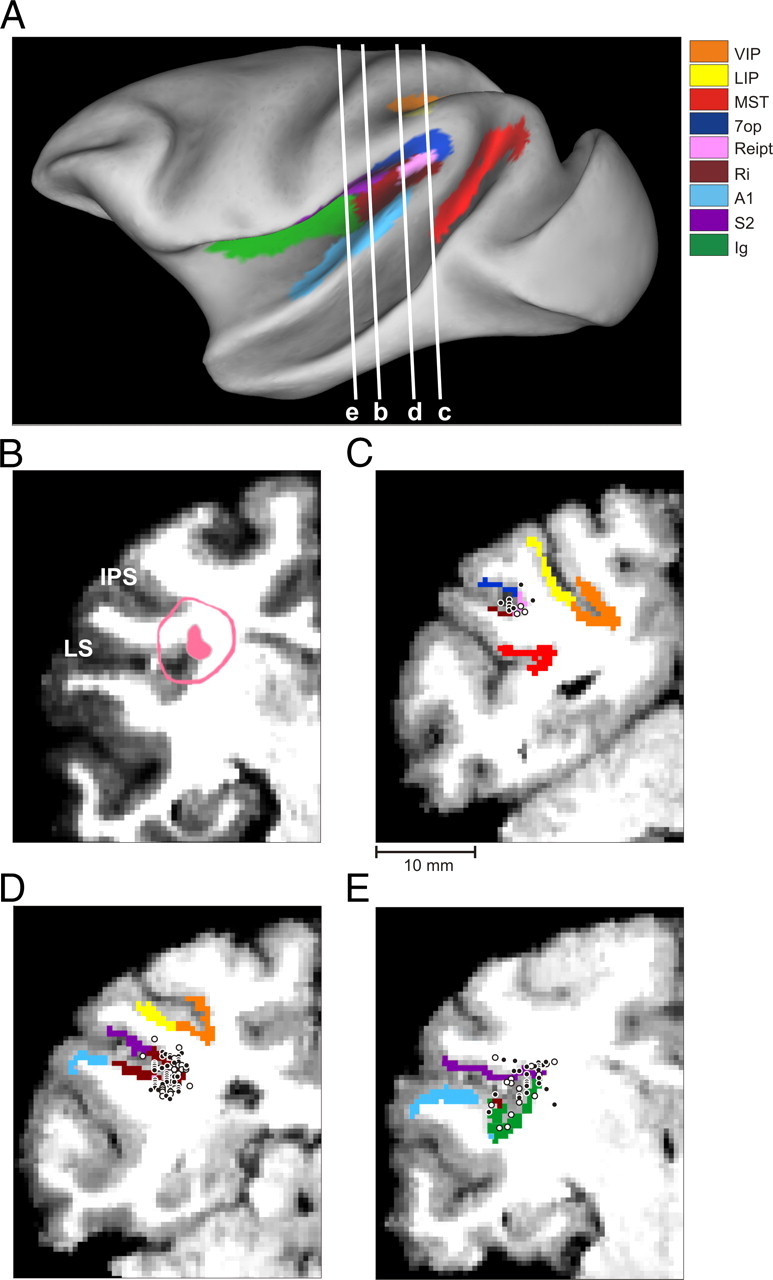
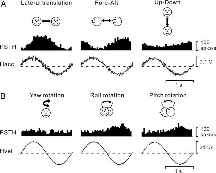
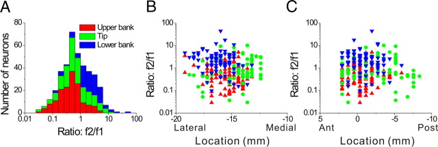
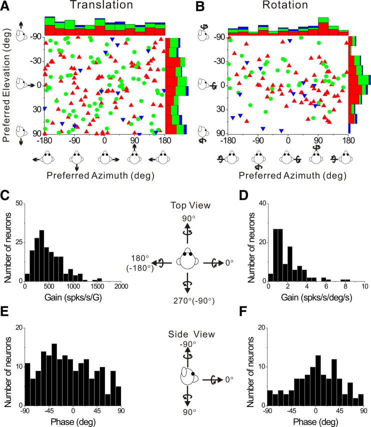
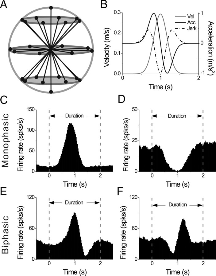
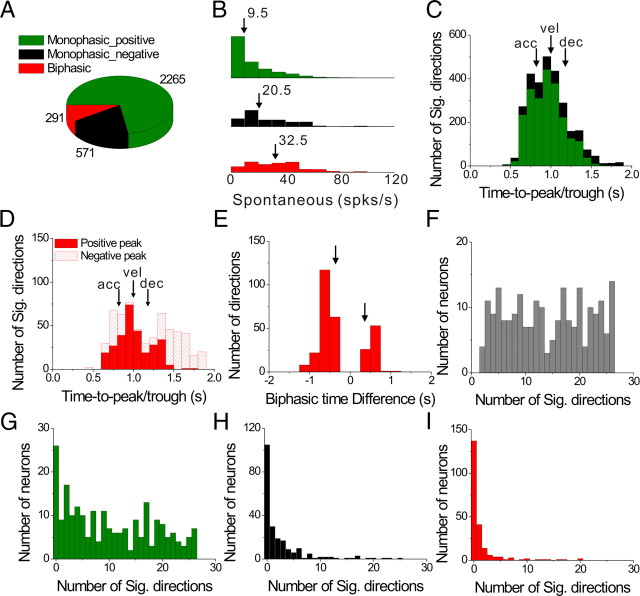
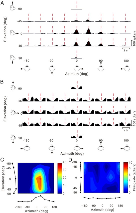
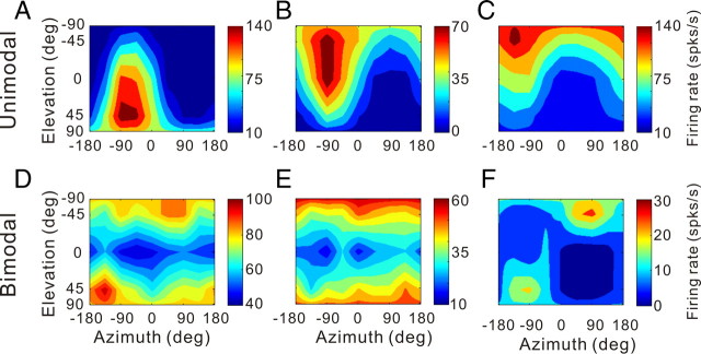
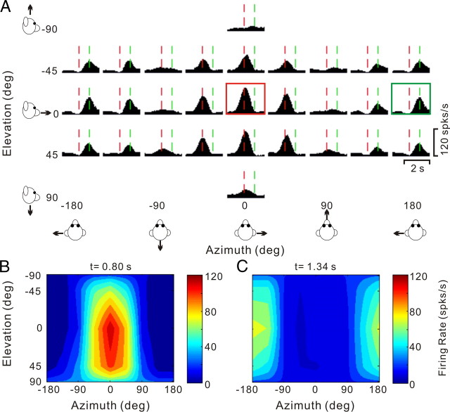
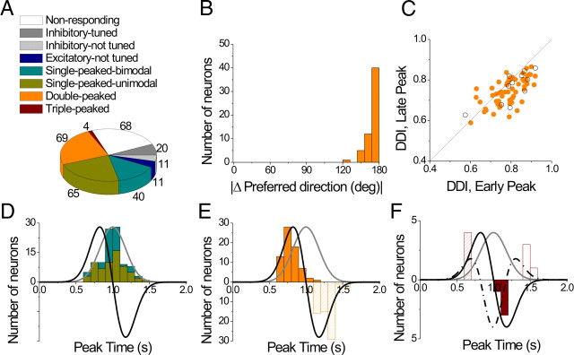
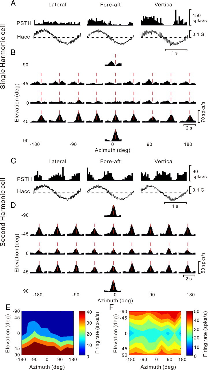
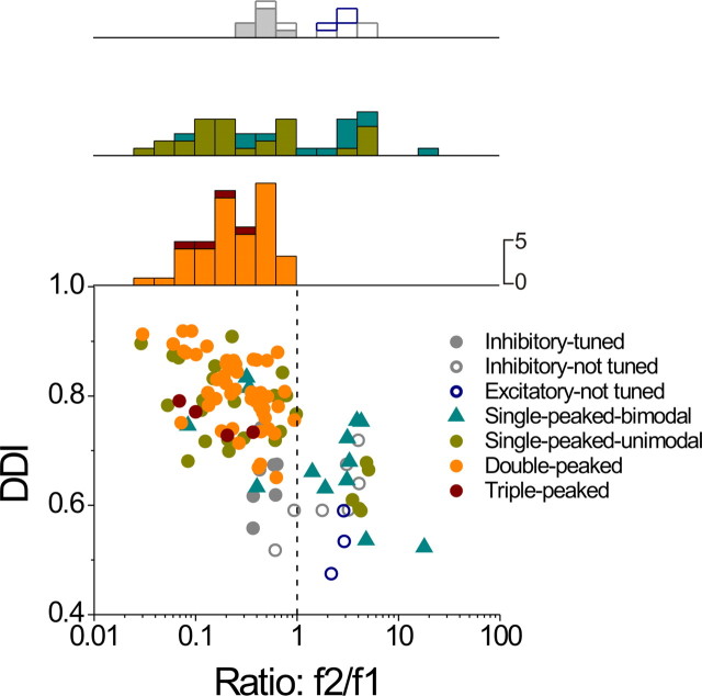
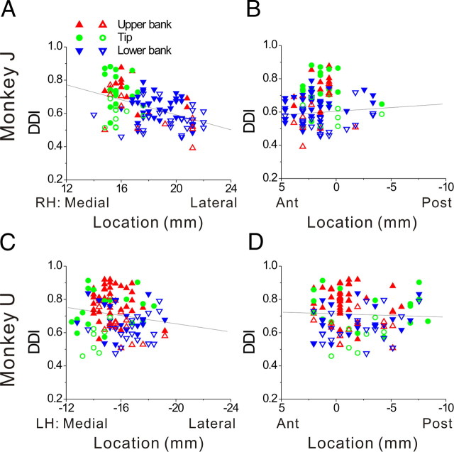
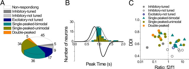
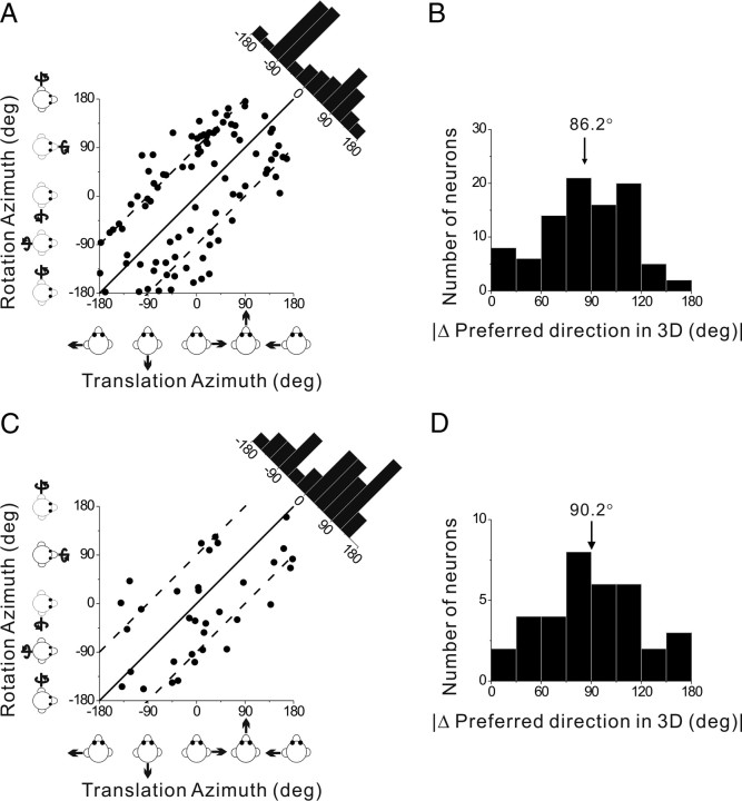
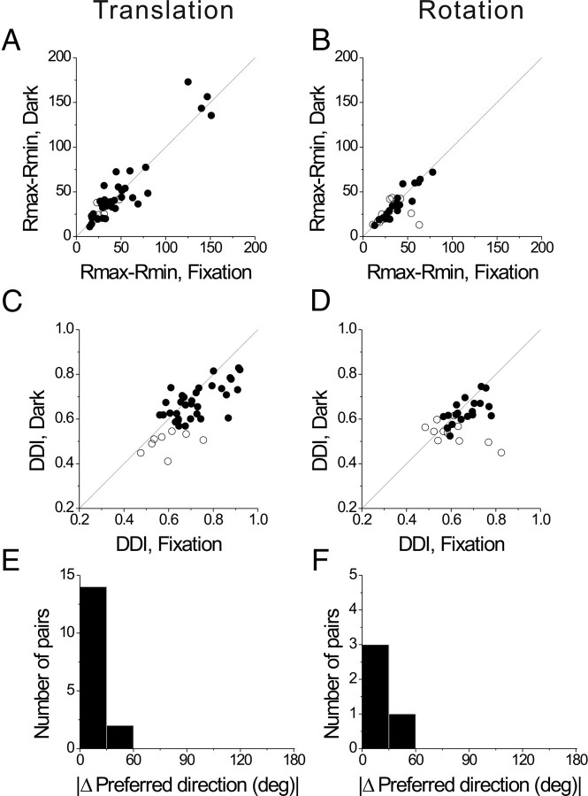
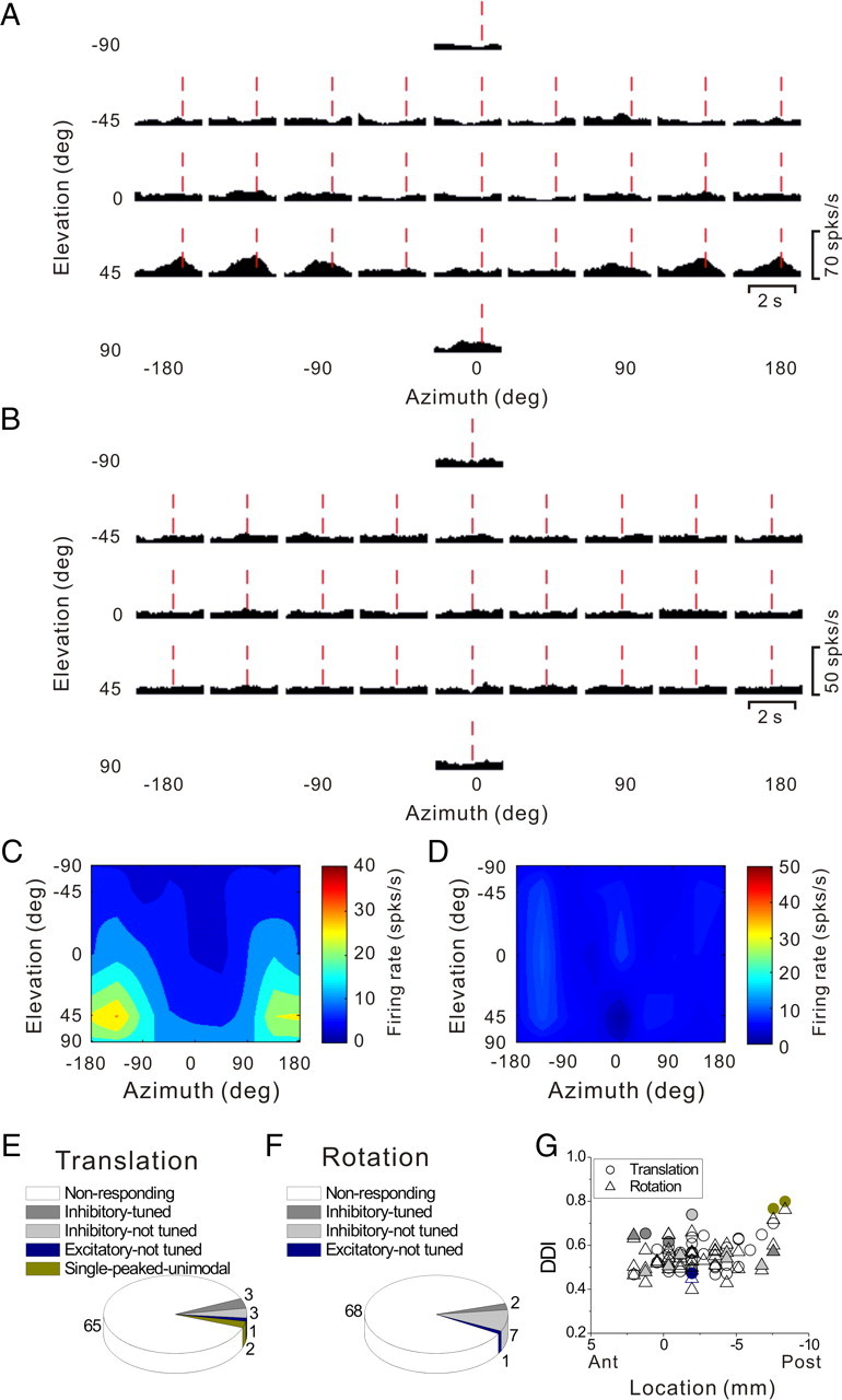
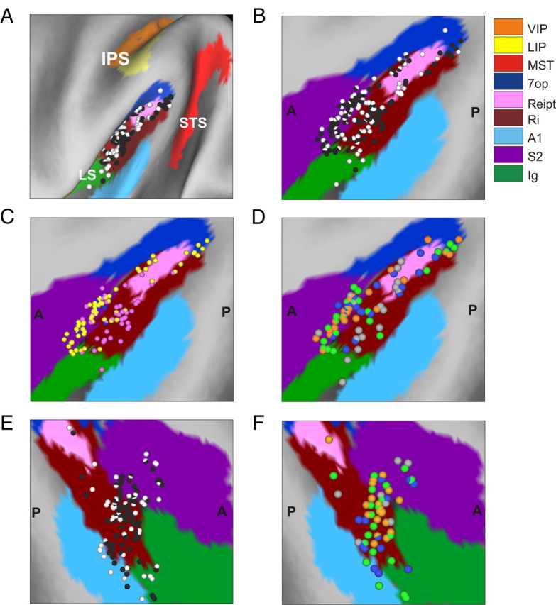
The parieto-insular vestibular cortex (PIVC) is thought to contain an important representation of vestibular information. Here we describe responses of macaque PIVC neurons to three-dimensional (3D) vestibular and optic flow stimulation. We found robust vestibular responses to both translational and rotational stimuli in the retroinsular (Ri) and adjacent secondary somatosensory (S2) cortices. PIVC neurons did not respond to optic flow stimulation, and vestibular responses were similar in darkness and during visual fixation. Cells in the upper bank and tip of the lateral sulcus (Ri and S2) responded to sinusoidal vestibular stimuli with modulation at the first harmonic frequency and were directionally tuned. Cells in the lower bank of the lateral sulcus (mostly Ri) often modulated at the second harmonic frequency and showed either bimodal spatial tuning or no tuning at all. All directions of 3D motion were represented in PIVC, with direction preferences distributed approximately uniformly for translation, but showing a preference for roll rotation. Spatiotemporal profiles of responses to translation revealed that half of PIVC cells followed the linear velocity profile of the stimulus, one-quarter carried signals related to linear acceleration (in the form of two peaks of direction selectivity separated in time), and a few neurons followed the derivative of linear acceleration (jerk). In contrast, mainly velocity-coding cells were found in response to rotation. Thus, PIVC comprises a large functional region in macaque areas Ri and S2, with robust responses to 3D rotation and translation, but is unlikely to play a significant role in visual/vestibular integration for self-motion perception.

Figure 1.

Anatomical localization of recording sites in the left hemisphere of monkey U. A, Inflated cortical surface illustrating the coronal sections drawn in B–E. B, A coronal MRI image showing portions of the LS and intraparietal sulcus (IPS). The filled pink region shows the dense core of signal produced by a manganese injection into the upper bank of the lateral sulcus, at a location where vestibular responses were identified physiologically. The outer pink contour shows the boundaries of the halo of less intense signal surrounding the injection. Manganese-induced responses have been superimposed on the baseline MRI image for this animal (see Materials and Methods). C–E, Coronal sections, spaced 4 mm apart, are shown from posterior (C) to anterior (E); cells located within 2 mm of each section were projected onto that section. Filled symbols with white borders represent single units that showed clear responses during sinusoidal translation and/or rotation, whereas open symbols with black borders illustrate cells that showed no response.

Figure 2.

A, B, PSTHs (averaged over multiple cycles) from an example neuron during 0.5 Hz sinusoidal translation (A) and rotation (B). Motion directions are indicated by the cartoon drawings. Stimulus traces shown represent linear acceleration (Hacc, A) or angular velocity (Hvel, B) of the head. The cell's response modulated significantly during all three translation directions, namely, lateral (708.1 spikes/s/G, p_{_f1} < 0.01, f2/f1 = 0.029), fore–aft (546.8 spikes/s/G, p_{_f1} < 0.01, f2/f1 = 0.114), and up–down (286.6 spikes/s/G, p_{_f1} < 0.01, f2/f1 = 0.159) motions. The cell also modulated significantly during roll (1.9 spikes/s/°/s, p_{_f1} < 0.01, f2/f1 = 0.236) and pitch (1.2 spikes/s/°/s, p_{_f1} < 0.01, f2/f1 = 0.409) rotations, but not during yaw rotation (p_{_f1} > 0.01 and p_{_f2} > 0.01).

Figure 3.

Relationship between the f2/f1 ratio (second/first harmonic of response modulation along the preferred direction of translation) and cell location within the lateral sulcus. A, Distribution of f2/f1 ratio (n = 420), plotted separately for cells recorded in the upper bank (red, n = 153), tip (green, n = 150), and lower bank (blue, n = 117) of the lateral sulcus. B, C, Scatter plots of the f2/f1 ratio as a function of medial–lateral and anterior–posterior stereotaxic coordinates. Only cells from the left hemisphere of monkey U (n = 273) are shown. Results were qualitatively consistent for monkey J, but not included here because sinusoidal responses were not saved for off-line analysis in many experiments (see Materials and Methods). Data are color-coded according to their location within the upper bank (red triangles), tip (green circles), and lower bank (blue triangles).

Figure 4.

Summary of sinusoidal responses. A, B, Distributions of direction preferences for translation (n = 185) and rotation (n = 114), in spherical coordinates (scatter plots of elevation versus azimuth preferences). Uniform azimuth and elevation distributions reflect direction preferences that are uniformly distributed on a sphere. The data are plotted on Cartesian axes that represent the Lambert cylindrical equal-area projection of the spherical stimulus space. Histograms along the top and right sides of each scatter plot show the marginal distributions. Data are color-coded based on the location of cells in the upper bank (red), tip (green), and lower bank (blue) of the lateral sulcus. C, D, Distributions of neural response gain along the 3D preferred direction for translation and rotation, respectively. E, F, Distributions of neural response phase along the 3D preferred direction for translation and rotation, respectively. Only neurons with significant single harmonic responses (p_{_f1} < 0.01) along at least one motion direction are included.

Figure 5.

Transient stimuli and examples of responses. A, Schematic of the 26 movement trajectories evenly spaced in 3D, 45° apart in both azimuth and elevation. B, The 2 s translational motion stimulus: velocity (gray curve), acceleration (black curve) and jerk (dashed-dot curve). C, D, Example average PSTHs with monophasic-positive and monophasic-negative temporal response profiles, respectively. E, F, Example average PSTHs with biphasic responses. Dashed lines indicate the onset and offset of the stimulus.

Figure 6.

Summary of temporal response modulation during 3D transient translational motion. A, Prevalence of monophasic positive (green), monophasic negative (black) and biphasic (red) temporal modulation profiles for all responsive motion directions (p < 0.01) in 220 cells. B, Histograms of spontaneous firing rates for monophasic positive, monophasic negative and biphasic responses; differences between groups were statistically significant (p < 0.001, Wilcoxon signed-rank test). C, Distribution of peak latency for monophasic responses. Vertical arrows mark the times of peak stimulus acceleration (“acc,” at 0.82 s), velocity (“vel,” at 1 s), and deceleration (“dec,” at 1.18 s). D, Distributions of peak response latency for biphasic responses. Red filled bars represent peaks; red hatched bars represent troughs. E, Distribution of the time difference between the peak and trough of biphasic responses. Vertical arrows mark the corresponding timing differences between peak stimulus acceleration and deceleration. F, Distribution of the number of stimulus directions that elicit significant responses for each responding cell (n = 220). G–I, Distributions of the number of significant response directions, now separated for monophasic-positive (G), monophasic-negative (H), and biphasic (I) response profiles, respectively.

Figure 7.

Responses of two PIVC neurons to 26 directions of transient translational motion. Azimuth and elevation are defined as in Figure 4. A, Average response PSTHs for a single-peaked neuron. Vertical dashed red lines indicate the peak time (0.94 s) when the maximum response across directions occurred. B, Average response PSTHs for a neuron with inhibitory responses. Vertical dashed red lines indicate the peak time (1.2 s) when the minimum response across directions occurred. C, Color contour map showing 3D directional tuning (Lambert cylindrical projection) at peak time for the cell in A (DDI = 0.77). Tuning curves along the margins of the color map illustrate mean firing rates plotted versus elevation or azimuth (averaged across azimuth or elevation, respectively). D, Color contour map showing spatial tuning at peak time of the inhibitory neuron in B; the cell was not significantly direction–selective at the peak time (shown) nor at any other time during the 2 s duration of the motion stimulus.

Figure 8.

A–F, 3D translational direction tuning for six example neurons with unimodal (A–C) and bimodal (D–F) spatial tuning. Preferred directions (computed by vector sum) were [azimuth, elevation] = [−60.3, 36.0°], [−82.4, −43.4°] and [−138.2, −63.2°] for the unimodal cells in A–C, respectively (DDI = 0.88, 0.86, and 0.88, respectively). The corresponding DDIs for the bimodal cells in D–F were 0.64, 0.65, and 0.79.

Figure 9.

Spatiotemporal responses for a double-peaked neuron. A, Average PSTHs for each of 26 directions of translation. The PSTH in the red square illustrates the first response peak occurring at t = 0.80 s (vertical red lines); the PSTH in the green square illustrates a second response peak occurring at t = 1.34 s (vertical green lines). B, C, Color contour maps showing the 3D tuning at the two peak times indicated in A. The tuning for the first peak (red square in A) is shown in B, with a direction preference at azimuth −2.8° and elevation 14.4° (DDI = 0.92). The tuning for the second peak (green square in A) is shown in C, with a direction preference at azimuth −175.7° and elevation −2.6° (DDI = 0.86). The difference in direction preference between the two peaks is 166°.

Figure 10.

Responses of a triple-peaked neuron. A, Average PSTHs for the 26 motion directions. Green, red, and blue vertical lines mark three distinct peak times. B–D, Color contour maps showing 3D tuning at the three peak times in A. Preferred directions were [azimuth, elevation]: [−50.7, −67.1°] (B), [124.6, 60.1°] (C), and [−73.3, −58.7°] (D). The corresponding DDI values were 0.83, 0.77, and 0.75, respectively.

Figure 11.

Population summary of the spatiotemporal tuning in response to transient 3D translation. A, Categories of tuning among responsive cells (n = 220). B, Distribution of the 3D difference in preferred direction (|Δ Preferred direction|) between the two distinct spatial tuning peaks of double-peaked cells; data are shown for 58/69 double-peaked cells with direction tuning that was unimodal at both peak times. C, Scatter plot of the DDI characterizing the strength of directional tuning at the two peak times of double-peaked cells. Filled symbols represent cells with unimodal spatial tuning for both peak times (n = 58). Open symbols represent cells with bimodal spatial tuning for at least one of the peak times (n = 11). D, Distribution of peak times for single-peaked cells. Green bars: cells with unimodal spatial tuning (n = 65); cyan bars: cells with bimodal spatial tuning (n = 40). E, Distribution of peak times for double-peaked cells (n = 69). Solid and hatched bars indicate the first and second peak times, respectively. F, Distribution of peak times for triple-peaked cells (n = 4). Stimulus velocity (gray), acceleration (black) and jerk (dashed-dotted line) profiles are overlaid in D–F. Distributions of the second peak times for double-peaked and triple-peaked cells have reversed polarity (negative ordinate values) for illustrative purposes.

Figure 12.

A–F, Examples of cells with first harmonic (A, B, E) and second harmonic (C, D, F) responses, as tested during both sinusoidal and 3D transient translation protocols. A, Average response PSTHs of a double-peaked cell during sinusoidal translation (0.5 Hz); the cell modulated during fore–aft (198.4 spikes/s/G, p_{_f1} < 0.01, p_{_f2} > 0.01, f2/f1 = 0.2, middle) and up–down (250 spikes/s/G, p_{_f1} < 0.01, p_{_f2} > 0.01, f2/f1 = 0.4, right) motion but not lateral motion (p_{_f1} > 0.01, p_{_f2} > 0.01, left). Hacc, Head acceleration. B, Average response PSTHs during transient translation of the same double-peaked cell; red lines indicate the second peak time (1.2 s) when the maximum response across all directions occurred. C, Average PSTHs of a second harmonic cell, responding to all directions of sinusoidal translation, namely, lateral (p_{_f1} > 0.01, p_{_f2} < 0.01, f2/f1 = 4.9), fore–aft (p_{_f1} > 0.01, p_{_f2} < 0.01, f2/f1 = 4.6), and up–down (p_{_f1} > 0.01, p_{_f2} < 0.01, f2/f1 = 3.1). D, Average response PSTHs for transient stimuli, showing significant temporal modulation along most (21/26) directions. Vertical red lines illustrate peak time (0.96 s). E, Color contour map showing 3D tuning for the second peak time (DDI = 0.84) for the cell shown in A and B. The cell's tuning was unimodal (p_{_uni} > 0.05, modality test), with a preferred direction at azimuth −83.9° and elevation 76.9°.The spatial tuning for the first peak time (data not shown) was also unimodal (DDI = 0.78), with a preferred direction at azimuth 11.6° and elevation −53.8°. F, Color contour map showing 3D spatial tuning at peak time for the second harmonic cell shown in C and D; tuning was spatially bimodal (DDI = 0.72).

Figure 13.

Comparison between sinusoidal responses (f2/f1 ratio) and 3D tuning (DDI). Each point in the scatter plot corresponds to one cell, and symbol shape/color reflects its classification as inhibitory (tuned or not tuned, filled or open gray circles, respectively), excitatory but not tuned (open blue circles), excitatory single peaked (bimodal/unimodal, cyan triangles/green circles), double peaked (orange circles), or triple peaked (red circles). The top panels show the distribution of f2/f1 ratios for inhibitory (tuned and not tuned; gray bars) and excitatory not tuned cells (top histogram; blue bars), single-peaked cells (middle histogram; cyan and green bars), and double-peaked and triple-peaked cells (bottom histograms; orange and red bars, respectively).

Figure 14.

Relationship between tuning strength, as measured by DDI, and cell location within the lateral sulcus. A–D, Scatter plots of DDI (measured at the time when the maximum response across directions occurred) as a function of medial–lateral (A, C) and anterior–posterior (B, D) stereotaxic coordinates (shown in millimeters) for cells recorded in the right hemisphere (RH) of monkey J (top, n = 113) and the left hemisphere (LH) of monkey U (bottom, n = 122). To make the data more comparable between the two monkeys, the medial–lateral coordinates on the x-axis for monkey U (C) were reversed to run from positive to negative. Because of differences in placement of the recording grid, the anterior/posterior extent of the recordings was slightly different in animals J and U. Red symbols: upper bank; green symbols: tip; blue symbols: lower bank cells. Filled symbols indicate cells with significant spatial tuning during translation (ANOVA, p < 0.01). Open symbols denote cells that were either not spatially tuned (ANOVA, p > 0.01) or did not pass the criterion for significant temporal modulation.

Figure 15.

Population summary of the spatiotemporal responses to 3D rotation. A, Classification of responsive cells (n = 106). B, Distribution of the peak times for single-peaked cells. Green bars: cells with unimodal spatial tuning (n = 34); cyan bars: cells with bimodal spatial tuning (n = 36). C, Scatter plot of tuning strength (DDI at peak time) during transient rotation versus the f2/f1 ratio from sinusoidal rotation responses. Each point in the scatter plot corresponds to a cell, and symbol shape/color reflects its classification as inhibitory (tuned or not tuned, filled or open gray circles, respectively), excitatory but not tuned (open blue circles), excitatory single peaked (bimodal/unimodal, cyan triangles/green circles), or double peaked (orange circles).

Figure 16.

Comparison of direction preferences between translation and rotation. A, C, Scatter plots comparing azimuth preferences for rotation and translation, shown for sinusoidal (n = 92) and transient (n = 35) responses, respectively. Solid and dashed lines illustrate 0 and ±90° differences between the preferred directions, respectively. Marginal distributions along the diagonal show the difference in preferred azimuth between translation and rotation. B, D, Histograms of the absolute differences in 3D direction preference between rotation and translation for sinusoidal and transient responses, respectively. For double-peaked or triple-peaked cells, preferred direction was calculated at the peak time that yielded the strongest spatial tuning. Data are shown only for cells with significant single harmonic modulation (A, B) or significant unimodal spatial tuning (C, D) for both translation and rotation.

Figure 17.

A–F, Comparison of responses under conditions of complete darkness versus visual fixation, plotted separately for translation (A, C, E) and rotation (B, D, F). All comparisons were made at the peak time of fixation responses. A, B, Scatter plots of peak-trough response amplitudes (R_max − R_min) during translation (n = 41) and rotation (n = 31), respectively. C, D, Scatter plots of DDI for the same cells as in A and B. E, F, Distribution of the difference in preferred direction under conditions of fixation and darkness, shown for translation (n = 16) and rotation (n = 4), respectively. Only neurons with unimodal spatial tuning at peak time for both fixation and darkness conditions are included in this comparison.

Figure 18.

PIVC neurons are generally unresponsive to optic flow. A–D, Example PSTHs and direction tuning profiles for two cells, one that responded selectively to optic flow during the visual translation protocol (A, C; same cell as in Fig. 12A,B,E) and another that did not show any response to optic flow (B, D; same cell as in Fig. 12C,D,F). Vertical red dashed lines indicate the respective peak times (1.3 and 1.1 s, respectively). The cell in A and C had a preferred direction at azimuth −171.6° and elevation 54.6° (DDI = 0.74). The cell in B and D was not spatially tuned. E, F, Categorization of PIVC neurons by responses to optic flow simulating translation (n = 74) and rotation (n = 78). G, Scatter plot of visual DDI plotted as a function of the anterior–posterior coordinate of each electrode penetration (in millimeters). Data are shown for the left hemisphere of monkey U during translation (circles, n = 38) and rotation (triangles, n = 49). Color coding of data points is as described for E and F.

Figure 19.

Anatomical localization of recording sites within and around the lateral sulcus. A, Lateral view of a 3D surface reconstruction of the left hemisphere of monkey U, with cell locations mapped onto the surface and with the three major sulci (IPS, LS, and STS) identified. Each dot corresponds to a cell, with black and white dots showing cells that were responsive and nonresponsive to sinusoidal motion, respectively. B–F, show flat maps of the brain areas around the lateral sulcus for the left hemisphere of monkey U (B–D) and the right hemisphere of monkey J (E, F). Different functional brain areas are color-coded as indicated in the legend. The color scheme for the data points representing individual cells is as follows. A, B, E, Black dots: responsive cells; white dots: nonresponsive cells (sinusoidal testing). C, Yellow dots: cells responding at the first harmonic to sinusoidal stimuli; pink dots: second-harmonic cells; blue dots: cells responding at both the first and second harmonics (sinusoidal testing). D, F, Gray dots: inhibitory cells; green dots: single-peaked unimodal cells; blue dots: single-peaked bimodal cells and untuned excitatory cells; orange dots: double-peaked cells (transient translation testing).

References

1. Akbarian S, Berndl K, Grusser OJ, Guldin W, Pause M, Schreiter U. Responses of single neurons in the parietoinsular vestibular cortex of primates. Ann N Y Acad Sci. 1988;545:187–202. - PubMed
1. Akbarian S, Grüsser OJ, Guldin WO. Thalamic connections of the vestibular cortical fields in the squirrel monkey (Saimiri sciureus) J Comp Neurol. 1992;326:423–441. - PubMed
1. Akbarian S, Grüsser OJ, Guldin WO. Corticofugal connections between the cerebral cortex and brainstem vestibular nuclei in the macaque monkey. J Comp Neurol. 1994;339:421–437. - PubMed
1. Angelaki DE. Dynamic polarization vector of spatially tuned neurons. IEEE Trans Biomed Eng. 1991;38:1053–1060. - PubMed
1. Angelaki DE. Spatio-temporal convergence (STC) in otolith neurons. Biol Cybern. 1992;67:83–96. - PubMed
Publication types
MeSH terms
LinkOut - more resources