

Impact of the infection period distribution on the epidemic spread in a metapopulation model
- PMID: 20195473
- PMCID: PMC2829081
- DOI: 10.1371/journal.pone.0009371
Impact of the infection period distribution on the epidemic spread in a metapopulation model
Abstract
Epidemic models usually rely on the assumption of exponentially distributed sojourn times in infectious states. This is sometimes an acceptable approximation, but it is generally not realistic and it may influence the epidemic dynamics as it has already been shown in one population. Here, we explore the consequences of choosing constant or gamma-distributed infectious periods in a metapopulation context. For two coupled populations, we show that the probability of generating no secondary infections is the largest for most parameter values if the infectious period follows an exponential distribution, and we identify special cases where, inversely, the infection is more prone to extinction in early phases for constant infection durations. The impact of the infection duration distribution on the epidemic dynamics of many connected populations is studied by simulation and sensitivity analysis, taking into account the potential interactions with other factors. The analysis based on the average nonextinct epidemic trajectories shows that their sensitivity to the assumption on the infectious period distribution mostly depends on R0, the mean infection duration and the network structure. This study shows that the effect of assuming exponential distribution for infection periods instead of more realistic distributions varies with respect to the output of interest and to other factors. Ultimately it highlights the risk of misleading recommendations based on modelling results when models including exponential infection durations are used for practical purposes.
Conflict of interest statement
Figures
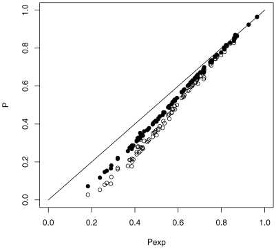
 refers to
  (closed circles) and
  (open circles). On x-axis Pexp refers to
  . For each of the three probabilities, 100 points with different parameter combinations were generated (
 and
and  were drawn from exponential distributions and
  was taken equal to 1). The points represent means over 100000 Monte-Carlo simulations of a time continuous event-driven approach: one infectious individual is introduced in one population and the probability of no secondary cases is calculated based on the time spent in each population. Estimated average standard deviation for computed values was below
  . All parameters and variables are explained in Table 1.
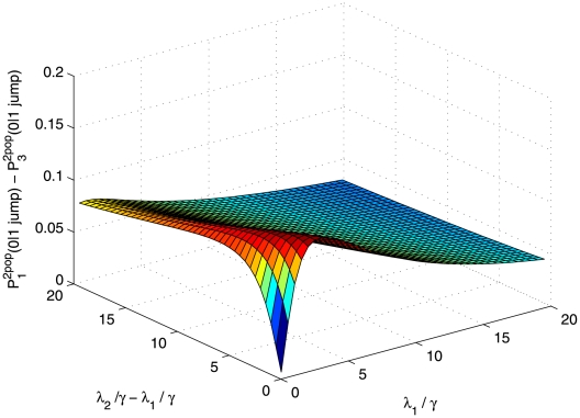
 is represented as a function of
  and
and  which vary on plausible ranges of values, under the constraint
  . All parameters and variables are explained in Table 1.
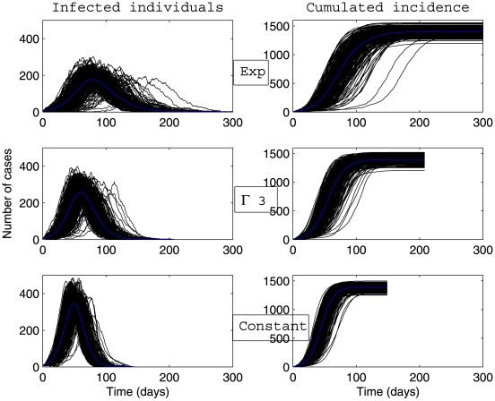
 ). Simulations are performed using a time-continuous event-driven approach with
  Exp(
Exp( ) (top panel),
  (middle panel) and
  (bottom panel). Parameters values are given in the subsection Examples of Results.
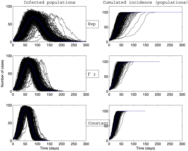
 ). Simulations are performed using a time-continuous event-driven approach with
  Exp(
Exp( ) (top panel),
  (middle panel) and
  (bottom panel). Parameters values are given in the subsection Examples of Results.
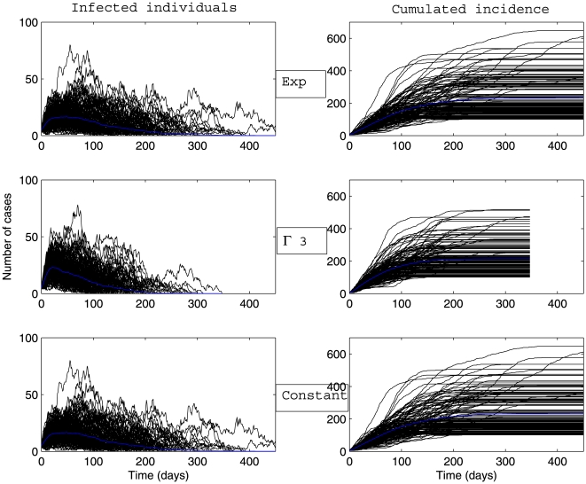
 ). Simulations are performed using a time-continuous event-driven approach with
  Exp(
Exp( ) (top panel),
  (middle panel) and
  (bottom panel). Parameters values are given in the subsection Examples of Results.
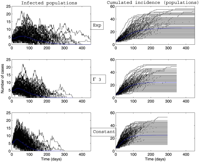
 ). Simulations are performed using a time-continuous event-driven approach with
  Exp(
Exp( ) (top panel),
  (middle panel) and
  (bottom panel). Parameters values are given in the subsection Examples of Results.
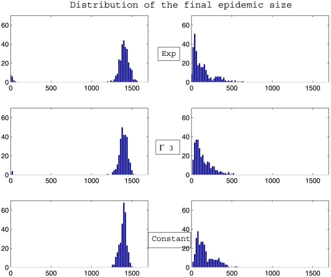
 Exp(
Exp( ) (top graphs),
  (middle graphs) and
  (bottom graphs). Parameters values are given at page 10.
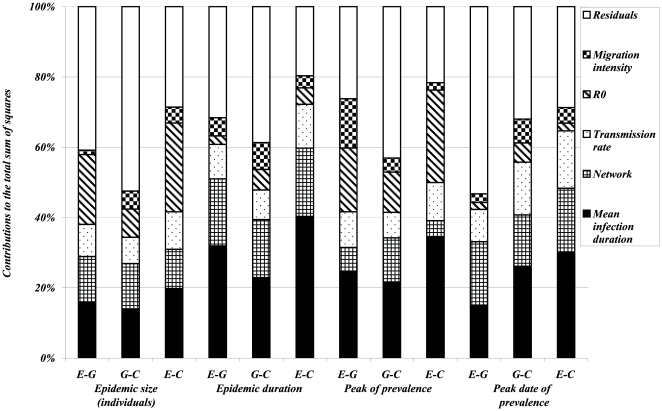
 (difference between the value of the output simulated with the exponentially distributed infectious period and the value corresponding to the gamma distributed infectious period),
  (difference between the value of the output simulated with the gamma distributed infectious period and the value corresponding to a constant infectious period) and
  (difference between the value of the output simulated with the exponentially distributed infectious period and the value corresponding to a constant infectious period). Different pattern fills correspond to contributions of five input factors (mean infection duration, network, transmission rate,
  and migration intensity) to the variation in outputs amongst scenarios.
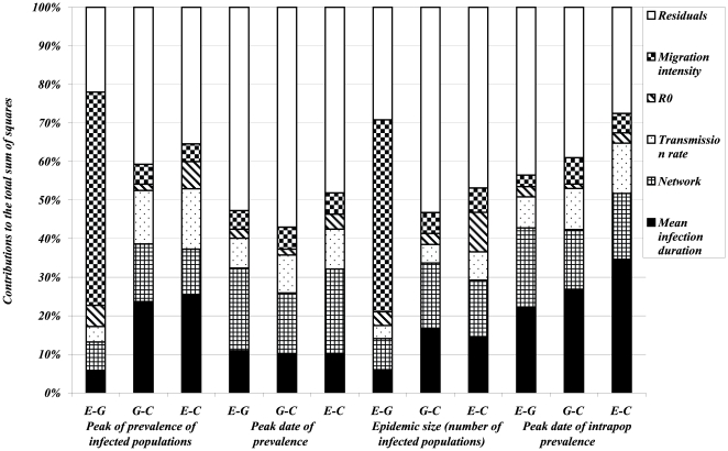
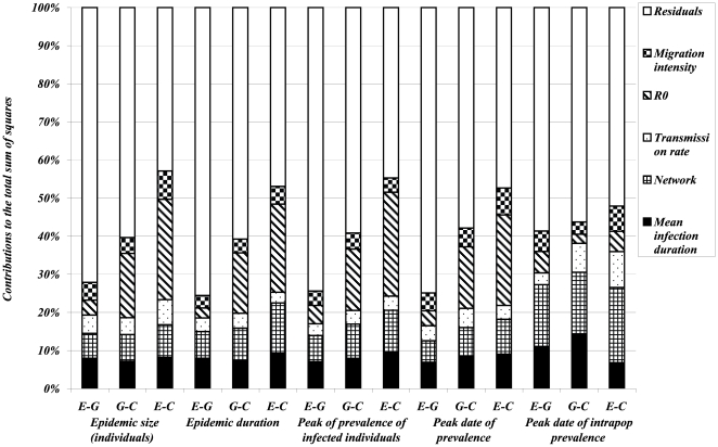
Similar articles
-
Illustration of some limits of the Markov assumption for transition between groups in models of spread of an infectious pathogen in a structured herd.Theor Popul Biol. 2008 Aug;74(1):93-103. doi: 10.1016/j.tpb.2008.05.002. Epub 2008 May 13. Theor Popul Biol. 2008. PMID: 18556035
-
Epidemic outbreaks on structured populations.J Theor Biol. 2007 Mar 7;245(1):125-9. doi: 10.1016/j.jtbi.2006.09.018. Epub 2006 Sep 23. J Theor Biol. 2007. PMID: 17097683
-
The effect of time distribution shape on a complex epidemic model.Bull Math Biol. 2009 Nov;71(8):1902-13. doi: 10.1007/s11538-009-9430-x. Epub 2009 May 28. Bull Math Biol. 2009. PMID: 19475454
-
The invasion, persistence and spread of infectious diseases within animal and plant communities.Philos Trans R Soc Lond B Biol Sci. 1986 Dec 15;314(1167):533-70. doi: 10.1098/rstb.1986.0072. Philos Trans R Soc Lond B Biol Sci. 1986. PMID: 2880354 Review.
-
Gaps in mobility data and implications for modelling epidemic spread: A scoping review and simulation study.Epidemics. 2023 Mar;42:100666. doi: 10.1016/j.epidem.2023.100666. Epub 2023 Jan 12. Epidemics. 2023. PMID: 36689876
Cited by
-
Testing, tracing and isolation in compartmental models.PLoS Comput Biol. 2021 Mar 4;17(3):e1008633. doi: 10.1371/journal.pcbi.1008633. eCollection 2021 Mar. PLoS Comput Biol. 2021. PMID: 33661888 Free PMC article.
-
Maternally Derived Immunity Extends Swine Influenza A Virus Persistence within Farrow-to-Finish Pig Farms: Insights from a Stochastic Event-Driven Metapopulation Model.PLoS One. 2016 Sep 23;11(9):e0163672. doi: 10.1371/journal.pone.0163672. eCollection 2016. PLoS One. 2016. PMID: 27662592 Free PMC article.
-
Fast and principled simulations of the SIR model on temporal networks.PLoS One. 2021 Feb 12;16(2):e0246961. doi: 10.1371/journal.pone.0246961. eCollection 2021. PLoS One. 2021. PMID: 33577564 Free PMC article.
-
Overcoming bias in estimating epidemiological parameters with realistic history-dependent disease spread dynamics.Nat Commun. 2024 Oct 9;15(1):8734. doi: 10.1038/s41467-024-53095-7. Nat Commun. 2024. PMID: 39384847 Free PMC article.
-
Modelling the key drivers of an aerial Phytophthora foliar disease epidemic, from the needles to the whole plant.PLoS One. 2019 May 28;14(5):e0216161. doi: 10.1371/journal.pone.0216161. eCollection 2019. PLoS One. 2019. PMID: 31136583 Free PMC article.
References
-
- Keeling MJ, Rohani P. Modeling infectious diseases in humans and animals. Princeton: Princeton University Press, first edition; 2008. 408
-
- Malice MP, Kryscio RJ. On the role of variable incubation periods in simple epidemic models. Math Med Biol. 1989;6:233–242. - PubMed
-
- Keeling MJ, Grenfell BT. Effect of variability in infectious period on the persistence and spatial spread of infectious diseases. Math Biosci. 1998;147:207–226. - PubMed
-
- Feng Z, Xu D, Zhao H. Epidemiological models with non-exponentially distributed disease stages and applications to disease control. Bull Math Biol. 2007;69:1511–1536. - PubMed
Publication types
MeSH terms
LinkOut - more resources
Full Text Sources
Medical
