Population genomics of parallel adaptation in threespine stickleback using sequenced RAD tags

Abstract

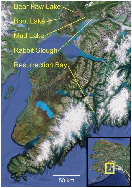
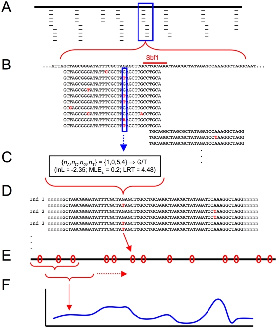
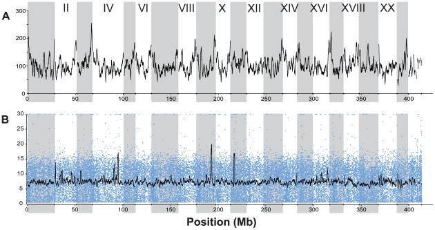
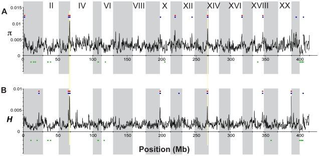
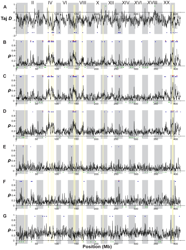
Next-generation sequencing technology provides novel opportunities for gathering genome-scale sequence data in natural populations, laying the empirical foundation for the evolving field of population genomics. Here we conducted a genome scan of nucleotide diversity and differentiation in natural populations of threespine stickleback (Gasterosteus aculeatus). We used Illumina-sequenced RAD tags to identify and type over 45,000 single nucleotide polymorphisms (SNPs) in each of 100 individuals from two oceanic and three freshwater populations. Overall estimates of genetic diversity and differentiation among populations confirm the biogeographic hypothesis that large panmictic oceanic populations have repeatedly given rise to phenotypically divergent freshwater populations. Genomic regions exhibiting signatures of both balancing and divergent selection were remarkably consistent across multiple, independently derived populations, indicating that replicate parallel phenotypic evolution in stickleback may be occurring through extensive, parallel genetic evolution at a genome-wide scale. Some of these genomic regions co-localize with previously identified QTL for stickleback phenotypic variation identified using laboratory mapping crosses. In addition, we have identified several novel regions showing parallel differentiation across independent populations. Annotation of these regions revealed numerous genes that are candidates for stickleback phenotypic evolution and will form the basis of future genetic analyses in this and other organisms. This study represents the first high-density SNP-based genome scan of genetic diversity and differentiation for populations of threespine stickleback in the wild. These data illustrate the complementary nature of laboratory crosses and population genomic scans by confirming the adaptive significance of previously identified genomic regions, elucidating the particular evolutionary and demographic history of such regions in natural populations, and identifying new genomic regions and candidate genes of evolutionary significance.

Figure 1. Location of oceanic and freshwater populations examined.

Threespine stickleback were sampled from three freshwater (Bear Paw Lake [BP], Boot Lake [BL], Mud Lake [ML]) and two oceanic (Rabbit Slough [RS], Resurrection Bay [RB]) populations in south central Alaska, USA (see inset). The three freshwater populations occur in different drainages and are separated by barriers to dispersal, and previous evidence supports the hypothesis that they represent independent colonization events from ancestral oceanic populations .

Figure 2. Schematic diagram of population genomic data analysis using RAD sequencing.

(A) Following Illumina sequencing of barcoded fragments, sequence reads (thin lines) are aligned to a reference genome sequence (thick line). Depth of coverage varies across tags. Reads that do not align to the genome, or align in multiple locations, are discarded. (B) Sample of reads at a single RAD site. The recognition site for the enzyme Sbf1 is indicated along the reference genome sequence (top), and sequence reads typically proceed in both directions from this point, at which they overlap. At each nucleotide site, reads showing each of the four possible nucleotides can be tallied (solid blue box). (C) Nucleotide counts at each site for each individual are used in a maximum likelihood framework to assign the diploid genotype at the site. In this example, G/T heterozygote is the most likely genotype; the method provides the log-likelihood for this genotype, a maximum-likelihood estimate for the sequencing error rate ε, and a likelihood ratio test statistic comparing G/T to the second-most-likely genotype, G/G homozygote. (D) Each individual now has a diploid genotype at each nucleotide site sequenced, and single nucleotide polymorphisms (SNPs, shown in red) can be identified across populations. Note, however, that haplotype phase is still unknown across RAD tags. (E) SNPs (red ovals) are distributed across the genome (thick line), and population genetic measures (e.g. F_ST) are calculated for each SNP. (F) A kernel smoothing average across multiple nucleotide positions is used to produce genome-wide distributions of population genetic measures.

Figure 3. Depth of RAD sequencing coverage.

(A) Number of RAD tags sequenced per 1-Mb sliding window across the genome. Each RAD tag represents either 30 or 47 bp of sequence data (see Table S1). Vertical gray shading indicates Linkage Groups I through XXI, followed by all unassembled scaffolds greater than 1 Mb in length. Not all RAD tags were sequenced in all individuals, because of both random sampling in the sequencing process and polymorphism in the restriction enzyme recognition site. (B) Sequencing depth per RAD tag per individual from one sample run (22 May 2009, lane 7; see Table S1). Blue dots represent the average number of reads per individual across 16 individuals sampled for each RAD tag. The black line shows the mean depth per individual in a 1-Mb sliding window. A total of 5,597,895 barcoded and aligned sequence reads from 16 individuals were generated from this run.

Figure 4. Genome-wide patterns of nucleotide diversity.

Each plot shows a smoothed distribution of the statistical measure across the genome (black lines). Colored bars above and below the distributions indicate regions of significantly elevated (p≤10⁻⁵, blue; p≤10⁻⁷, red) and reduced (p≤10⁻⁵, green) values, assessed by bootstrap resampling. Vertical shading indicates the 21 linkage groups and the unassembled scaffolds greater than 1 Mb in length, and gold shading indicates two regions showing evidence of balancing selection as discussed in the text. (A) Nucleotide diversity (π) across all five stickleback populations sampled. (B) Heterozygosity (H) across all five populations.

Figure 5. Evidence for balancing selection on Linkage Group III.

Population genetic measures plotted along Linkage Group III. (A) Nucleotide diversity (π) and (B) heterozygosity (H) across all five (blue), the three freshwater (red), and the two oceanic (green) populations. (C) Population differentiation (F_ST) between oceanic and freshwater (blue), among freshwater (red), and between oceanic (green) populations. Colored bars indicate significant (p≤10⁻⁵) regions of elevated (above the plots) or reduced (below the plots) values of each statistic for the corresponding set of populations. Vertical yellow shading indicates the region of putative balancing selection used for candidate gene annotation.

Figure 6. Genome-wide differentiation among populations.

F_ST across the genome, with colored bars indicating significantly elevated (p≤10⁻⁵, blue; p≤10⁻⁷, red) and reduced (p≤10⁻⁵, green) values. Vertical gray shading indicates boundaries of the linkage groups and unassembled scaffolds, and gold shading indicates the nine peaks of substantial population differentiation discussed in the text. (A) F_ST between the two oceanic populations (RS and RB; note that no regions of F_ST are significantly elevated or reduced). (B,C,D) Differentiation of each single freshwater population from the two oceanic populations, shown as the mean of the two pairwise comparisons (with RS and RB): (B) BP, (C) BL, (D) ML. Colored bars in each plot represent regions where both pairwise comparisons exceeded the corresponding significance threshold. (E) Overall population differentiation between the oceanic and freshwater populations. (F) Differentiation among the three freshwater populations (BP, BL, ML).

Figure 7. Differentiation among oceanic and freshwater populations on Linkage Groups I, II, and IV.

For each linkage group, the upper panel shows population differentiation (F_ST) of each freshwater population from the two oceanic populations, plotted as the mean of the two freshwater versus oceanic comparisons for each freshwater population: BP (blue), BL (red), ML (green). Colored bars indicate regions of bootstrap significance (p≤10⁻⁵) for the corresponding population. The lower panel shows F_ST for the overall oceanic-freshwater comparison (black), F_ST among the three freshwater populations (orange), and corresponding regions of significance (p≤10⁻⁵), along with F_ST values (blue circles) at single nucleotide polymorphisms at which population differentiation is significant at the level of α = 10⁻²⁰ in a G-test corrected for false discovery rate. Vertical shading indicates boundaries of the peaks used for candidate gene annotation. (A) LG I. (B) LG II. (C) LG IV.

Figure 8. Differentiation among oceanic and freshwater populations on Linkage Groups VII, VIII, XI, and XXI.

All panels show population differentiation as in Figure 7. (A) LG VII. (B) LG VIII. (C) LG XI. (D) LG XXI.

Figure 9. Genome-wide distributions of allele frequency spectrum and private allele density.

(A) Tajima's D, a measure of allele frequency spectrum, within the combined oceanic population (RS and RB). Colored bars above and below the distribution indicate regions of significantly elevated (p≤10⁻², green) or reduced (p≤10⁻², blue; p≤10⁻⁴, red) values, assessed by bootstrap resampling. (B–G) Private allele density (ρ) in single freshwater populations. Colored bars indicate regions of significantly elevated (p≤10⁻³, blue; p≤10⁻⁵, red) or reduced (p≤10⁻³) values. (B) Private allele density in BP relative to combined oceanic populations (OC). (C) BL relative to OC. (D) ML relative to OC. (E) Private allele density in BP relative to other freshwater populations (FW). (F) BL relative to FW. (G) ML relative to FW. Across all panels, vertical gray shading indicates Linkage Groups I-XXI and unassembled scaffolds, and gold shading indicates the nine peaks of population differentiation highlighted in Figure 7 and Figure 8.

References

1. Fisher RA. New York: Dover; 1958. The Genetical Theory of Natural Selection.
1. Wright S. Chicago: University of Chicago Press; 1978. Evolution and the genetics of populations.
1. Kimura M, Ota T. Theoretical aspects of population genetics. Monogr Popul Biol. 1971;4:1–219. - PubMed
1. Gillespie JH. The status of the Neutral Theory: The Neutral Theory of Molecular Evolution. Science. 1984;224:732–733. - PubMed
1. Charlesworth B. Effective population size and patterns of molecular evolution and variation. Nat Rev Genet. 2009;10:195–205. - PubMed
Publication types